Born image perturbation

The simplest way of computing image/wavefield perturbations is by simple subtraction of the wavefields for the background image $\mathcal U_o$from the wavefield of a better image $\mathcal U$: 

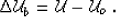$$\Delta \mathcal U_b= \mathcal U- \mathcal U_o\;.$$ (13)

Equation (13) is only valid for small perturbations of the wavefields ($\Delta \mathcal U_b<< 1$). In practice, this requirement means that the cumulative phase difference between the two different wavefields is small at all frequencies.

If this condition is satisfied, we can compute a slowness perturbation which corresponds to the Born approximation:  

$$\Delta s_b= {\bf B}^* \left(\mathcal U_o\right)\left[\Delta \mathcal U_b\right]\;.$$ (14)

In practice, the small perturbation requirement is hard to meet, since small slowness differences ammount to large cumulative phase differences. Thus, with the wavefield perturbation definition in equation (13), we can only handle small slowness perturbations.