AVA analysis

For the AVA analysis I chose the simple slope*intercept (A*B) methodology used in Castagna et al. (1998); Gratwick (2001). Figure 11 shows the slope (left), intercept (center), and slope*intercept (right) for the migrated image without model variability. Note the positive, hydrocarbon indicating, anomalies circled at approximately 2.3 km.

 

ava-none
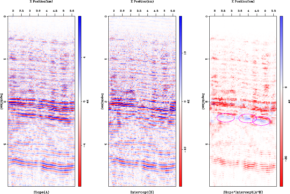
Figure 11 AVA analysis for the migrated image in Figure 7. The left panel shows the slope, the center the intercept, and the right panel the slope*intercept.

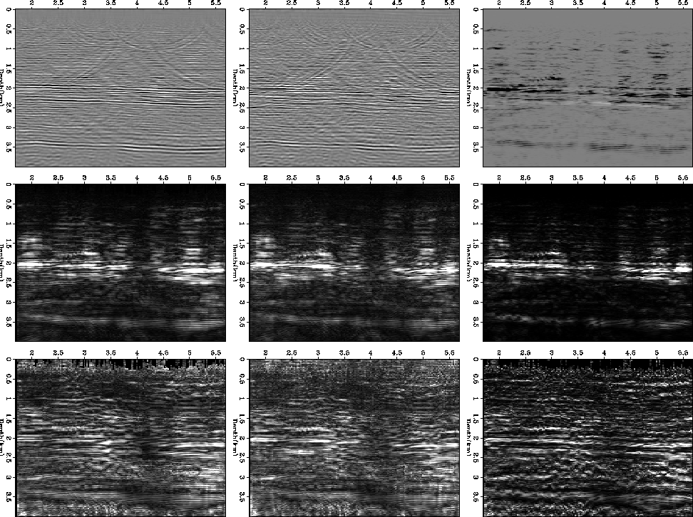
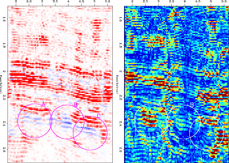
I then performed the same procedure on all of the migrated images obtained from the various realizations (Figure 12). The left panel shows intercept, the center panel slope, the right panel, slope*intercept. The top shows the average of the realizations. The center panel shows the variance of the realizations. The bottom panel shows the variance scaled by the inverse of the smoothed amplitude. What is interesting is the varying behavior at the three zones with hydrocarbon indicators. Figure 13 shows a closeup in the zone with the hydrocarbon indicators. The left blob `A' shows a high variance in the AVA indicator. The center blob `B' shows a mild variance, and the right blob `C' shows low variance. This would seem to indicate that at location `C' the hydrocarbon indicator is more valid. Without drilling of each target a more general conclusion cannot be drawn.

 

ava-multi
Figure 12 AVA analysis for the the various velocity realizations. The left panel shows intercept, the center panel slope, the right panel, slope*intercept. The top shows the average of the realizations. The center panel shows the variance of the realizations. The bottom panel shows the variance inverse scaled by a smoothed amplitude.

 

ava-multi-close
Figure 13 A close up of the reservoir zone. The left panel shows the slope*intercept. The right panel shows the variance of the slope*intercept for the various realizations. Note how the left blob `A' shows a high variance in the AVA indicator. The center blob `B' shows a mild variance, and the right blob `C' shows low variance.

Conclusions I showed how AVA parameter variability can be assessed by adding a random component to our fitting goals when estimating velocity. The methodology shows promise in allowing error bars to be placed upon AVA parameter estimates.

I would like to thank Ecopetrol for the data used in this paper.