Introduction

To build a velocity stack, we usually construct an operator ${\bf H}$that maps energy from velocity-stack space to offset-travel time space. The adjoint operator ${\bf H'}$ maps the energy back to a velocity-stack space. To build the model in a $\tau-s$ domain that is consistent with the data, we then solve the least-squares problem:

$$\begin{eqnarray} \bf Hm - d &\approx& \bf 0\end{eqnarray}$$ (1)

This problem can be solved using iterative methods. For a simple model the solution is usually obtained in a few iterations. Although this solution may fit the data well, it may have ``butterfly'' artifacts caused by a limited aperture of the data. To illustrate this, I create a simple model with one spike in the velocity-stack space. Applying the operator ${\bf H}$ to this model, I obtain synthetic data set. Then I use this modeled data as an input (${\bf d}$) to solve the least-squares problem (equation 1) for ${\bf m}$.Figure 1 shows the original model in the velocity-stack space, the modeled data, the estimated model, and data residual after five iterations of the conjugate gradient method.

 

spike
Figure 1 Top left: Ideal model. Top right: Spike after 5 iterations of the conjugate gradient. Bottom left: Data modeled from the ideal model. Botton right: Data residual after 5 iterations

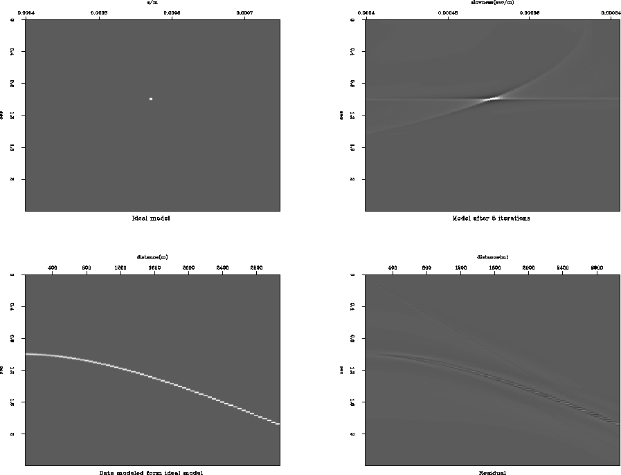
As Figure 1 shows, the data residual after five iterations is small but ``butterfly'' artifacts are clearly present in the solution. It is desirable to obtain a model that has all the energy concentrated at the location of the original spike and fits the data well. This problem has been addressed before. For example, at SEP Nichols (1994) and Guitton (2000) proposed to minimize the L1 norm of the model to create the spiky solution. Sacchi and Ulrych (1995) solved a similar problem using a parabolic Radon trasform, where they solve the problem in a frequency domain. These techniques showed very good results in concentrating the energy of the solution. (They are especially valuable during the multiple attenuation step of the processing.) But for some applications it may be useful to have an inexpensive way to remove artifacts from the model even if the data residual becomes larger. My first goal is to use the spatial predictability of the artifacts to design the operator to remove them. If the technique can make events appear better in a velocity stack panel and is easy to apply, it can be useful in picking velocities and designing masks for a multiple removal. A similar approach may be effective in other geophysical applications where the artifacts have a similar nature; for example, artifacts caused by a limited apperture in Kirchhoff migration.