Space variable damping in conventional imaging condition

Conventional shot profile migration schemes determine the reflection strength at each subsurface point taking into account only the downgoing and the upgoing wavefields at that location. Jacobs (1982) compares two different imaging conditions  

$$\bf r=\sum_{t} ud,$$ (7)

and  

$$\bf r=\sum_{t}\frac{ ud}{ d^2+\varepsilon^2}.$$ (8)

The first is one commonly used by the industry. It has the advantage of being robust, but has the disadvantage of not computing the correct amplitudes. The second computes the correct amplitudes (except for a damping factor $\varepsilon$), but has the disadvantage of being unstable due to zero division. That is why a damping factor $\varepsilon$ is needed.

We propose to add a mask function defined as  

$$\bf w=\left\{ \begin{array} {c} 0 \quad \mbox{if} \quad \bf... ...t \alpha \\ 1 \quad \quad \mbox{otherwise} \end{array}\right.$$ (9)

where $\alpha$ can be variable in space.

When $\bf ud$ has enough energy to contribute to the image, the damping factor $\varepsilon$ is set to zero. When factor $\bf ud$ is small, the damping factor is kept to avoid zero division. Thus, the imaging condition can be set as  

$$\bf r=\sum_{t}\frac{ ud}{ d^2+w \varepsilon^2},$$ (10)

where the damping is now variable in space.

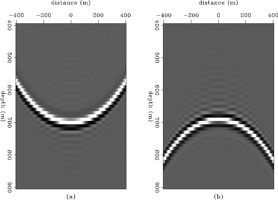
A simple synthetic was generated to test the preceding idea using wave equation modeling. Figure 3a shows the downgoing wave, and Figure 3b the upgoing wave, at a fixed time. Figure 4 shows the mask $\bf w$ used in this example.

 

DU
Figure 3 Wavefields at a fixed time. a) Downgoing wave, b) Upgoing wave.

 

ma
Figure 4 Mask used in equation (10). Zero at masked area and one out of the masked area.

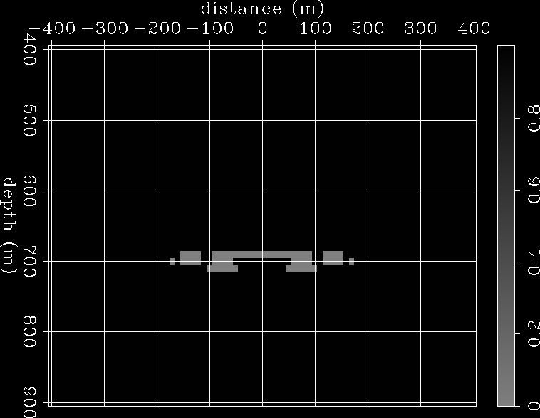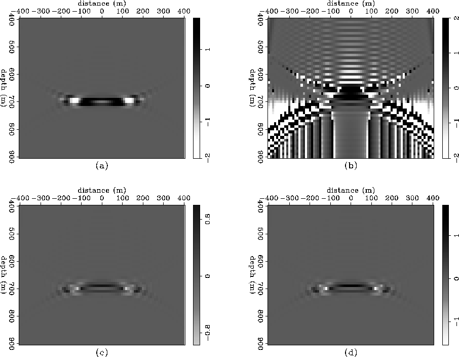
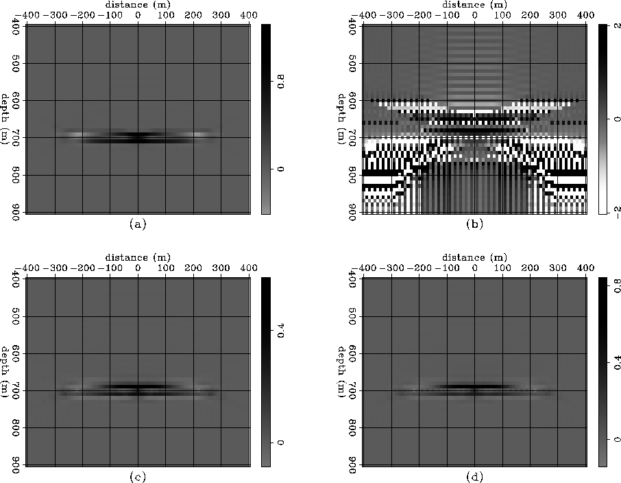
Figure 5a shows the reflection strength calculated using the imaging condition stated in equation (7). Figure 5b shows the reflection strength calculated using division of the upgoing wavefield $\bf u$ by the downgoing wavefield $\bf d$. Figure 5c shows the reflection strength calculated using the imaging condition stated in equation (8), and Figure 5d shows the reflection strength calculated using the imaging condition stated in equation (10). The advantage of Figure 5d's result over the others is that it has the correct reflection strength value inside the masked area and doesn't diverge outside it because of the damping factor.

 

comp_1shot
Figure 5 Comparison between four different imaging conditions a) Calculated by wavefield multiplication equation (7), b) Calculated by wavefield division ($\bf ud$), c) Calculated using constant damping equation (8), and d) Calculated using space variable damping equation (10).

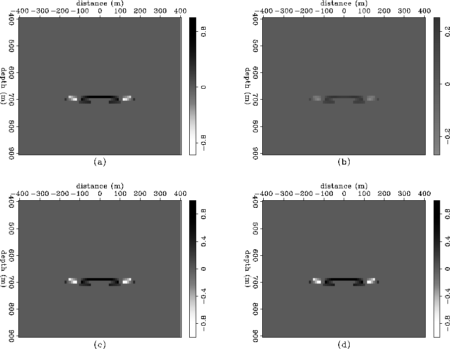
In Figure 6 we compare the two imaging conditions stated in equations (8) and (10) inside the masked area for two different $\varepsilon$. We can see for the imaging condition stated in equation (10) that the reflection strength inside the masked area doesn't change. This is an important advantage of space variable damping imaging principle, because it let us to build an adaptive mask dependent of the subsurface illumination.

 

comp_im
Figure 6 Comparison between imaging condition stated in equations (8) and (10) inside the masked area. a) $\varepsilon=0.5$, b) $\varepsilon=5$, c) $\varepsilon=0.5$, d) $\varepsilon=5$

We stack the reflection strength from 11 shots to see how the change observed in one shot affects the final image. The result is shown in Figure 7. We can see imaging condition from equation (10) gives the best resolution.

 

comp_stack
Figure 7 Comparison between 11 shot stacks using three different imaging conditions, a) equation (7), b) wavefield division ($\bf ud$), c) equation (8), and d) equation (10).