Implementation of a wave simulator

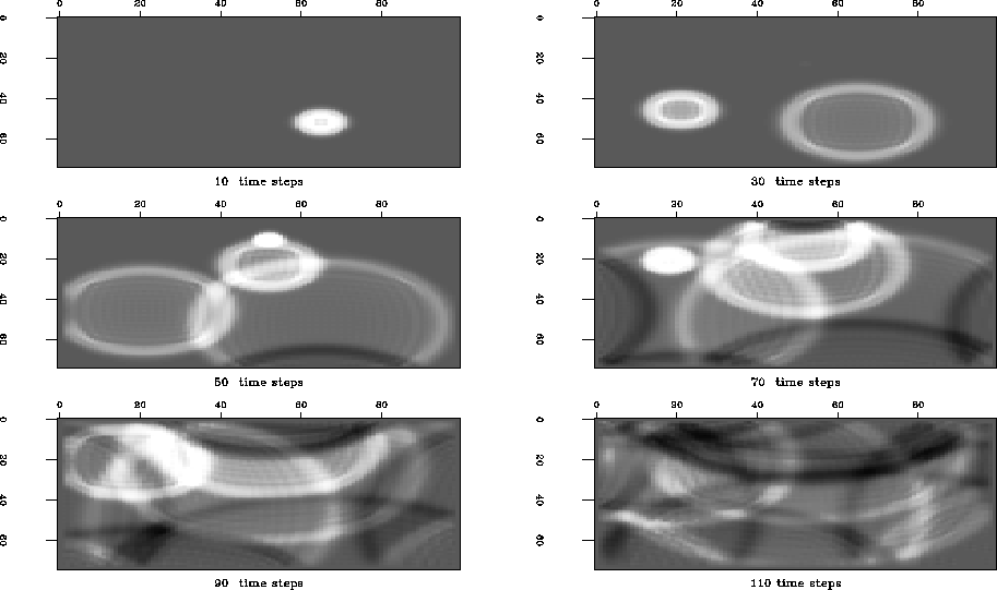
I implemented a finite-difference simulator for the rudimentary acoustic two-way wave equation 10. For my preliminary exploits, I chose a 2-D plane. The finite difference simulator computes the wavefield for arbitrarily placed sources. I intend to first model simple transmission experiments, possibly with plane waves. Seismogramms for various acquisition geometries are easily extracted from the complete wavefield.

Following Gassmann's model, the fluid saturated, porous rock properties enter the simulator by defining the velocity field v of equation 11. In particular, Gassmann's bulk modulo and density depend on the fluid saturation S_o, S_w and S_g. I assume that the fluid flow in a producing reservoir and the wave propagation of a seismic experiment are decoupled, since both processes happen on very different time scales and are limited to small, linear motions. Consequently, I assume the saturation and the dependent velocity as fixed during a seismic experiment. However, I expect that the saturation and consequently the velocity of the reservoir rocks possibly changes between subsequent experiments.

I implemented the finite difference simulator as part of Jest Schwab and Schroeder (1997), a Java inversion library. The linear simulators contain their adjoint operator that are checked by the dot product test.

Finite difference wave equation. I implement the acoustic scalar wave equation  

$$\ddot{\sigma} = v^2 \nabla^2 \sigma$$ (18)

as a finite difference formula which is second-order accurate in space and time

$$\sigma_{t+1}^{x,y} - 2 \sigma_t^{x,y} + \sigma_{t-1}^{x,y} =... ...) + (\sigma_t^{x,y-1} -2 \sigma_t^{x,y} + \sigma_t^{x,y+1})]$$

where $\hat{v} = v \Delta t / \Delta x$. Isolation of $\sigma_{t-1}^{x,y}$ and addition of identical terms yields the final difference formula  

$$\sigma_{t+1}^{x,y} = (2 - 4 \hat{v}^2) \sigma_t^{x,y} + \ha... ... (\sigma_t^{x,y-1} + \sigma_t^{x,y+1})] - \sigma_{t-1}^{x,y}.$$ (19)

The Figure 4 shows snapshots of a constant velocity wavefield that is excited by random point sources.

Boundary conditions. I also implemented Clayton and Engquist's 1980 absorbing boundary conditions. The absorption of the wave is due to a subtle change of the material coefficients at all edge points of the computational grid. While the interior coefficients implement the two-way wave equation, the boundary points implement the paraxial one-way wave equation. The one-way wave equation propagates the energy outwards but not inwards. Unfortunately, I am currently baffled since my implementation does not absorb the energy as promised.

 

impWaveSnap
Figure 4 Snapshots of the acoustic wave equation simulator for a constant propagation medium and randomly located point sources. The panels show a wavefield as time increases from left to right and top to bottom. An impulsive source generates an impulse that propagates spherical wavefronts (Scaling of the image might make the wavefront appear elliptical). The wavefront is reflected at the boundary.

Stability analysis. The fundamental solution to the difference equation above is

$$\sigma_t^{x,y} = \xi^t e^{i k_x j \Delta x} e^{i k_y l \Delta y} \sigma_0.$$ (20)

The value of $\xi$ has to be less or equal 1 to ensure that the solution does not grow exponentially with t (Courant-Friedrichs-Levy condition). Substitution of the fundamental solution into the difference equation 19 yields

$$0 = \xi^2 + [(2-4\hat{v}^2) + \hat{v}^2(e^{- i k_y \Delta y}... ...} + e^{ i k_x \Delta x} + e^{- i k_x \Delta x})] \xi + 1.$$ (21)

This equation is a quadratic polynomial in $\xi$. The quadratic has a real solution only if its determinant is greater or equal than . Since

$$e^{-i \phi} + e^{i \phi} = 2 \cos{\phi}$$

we can write the determinant as

$$0 \leq [2 (1 + 2 \hat{v}^2 (u-1)]^2 - 4$$

where $u = (1/2) (\cos{k_x \Delta x} + \cos{k_y \Delta y}) \in [-1,1]$. Isolation of $\hat{v}^2$ leads to

$$\frac{1}{2} \geq \hat{v}^2$$

where we divided once by $(u-1) \le 0$. In summary, the finite difference computation is stable as long as $\hat{v} = v \Delta t / \Delta x$ is smaller than $1/\sqrt{2}$.This expression might be used to choose $\Delta t$ for a given velocity v and a desired output interval $\Delta x$.

Implementation. The finite difference equation 19 expresses a recursive computation in time of the wavefield $\sigma$ over time:  

$${\bf \sigma}_t = a {\bf \sigma}_{t-1} + b {\bf \sigma}_{t-2} + {\bf s}_t$$ (22)

where ${\bf s}_t$ is the known source contribution at time t. The vectors ${\bf \sigma}_t$ and ${\bf s}_t$ refer to constant time instances of the spatial (x,y) grid. The equation expresses only the time dependency of the recursion explicitly: the straightforward spatial convolution of the original finite difference equation is symbolically represented by the coefficients a and b.

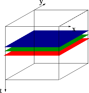
Figure 5 indicates how the algorithm recursively computes the values in the red plane from the earlier green and blue plane. The first two time planes implement the initial conditions. Once the entire cube is computed, a constant time plane contains a snapshots of the wavefield. The extraction of all wavefield values that correspond to a (x,y)-location yields a time dependent seismogram.

 

cube Figure 5 Computational grid. The domain and range of the finite difference implementation is an identical cube of (x,y,t) values. The input cube contains the source amplitudes of any point in time and space. The output cube contains the wavefield amplitude of any point in time and space. The values in the red plane are computed from the values of the green and blue plane according to the difference equation 19.

The recursion 22 is a handy approach to compute the wave solution ${\bf \sigma}$ of the fundamental operator equation  

$${\bf A} {\bf s} = {\bf \sigma}.$$ (23)

Because of the operator's recursive definition, we do not know its explicit matrix form ${\bf A}$. However, the recursion 22 is easily reformulated to

$${\bf s}_t = {\bf \sigma}_t - a {\bf \sigma}_{t-1} - b {\bf \sigma}_{t-2}$$

which corresponds to the matrix expression ${\bf s} = {\bf A}^{-1} {\bf \sigma}$ or  

$$\left[ \begin{array} {c} s_0 \\ s_1 \\ s_2 \\ s_3 \\ \end{ar... ...ma_0 \\ \sigma_1 \\ \sigma_2 \\ \sigma_3 \\ \end{array}\right].$$ (24)

In summary, we have a recursive formula to compute ${\bf \sigma}$ from ${\bf s}$ but we lack a simple explicit matrix expression. On the other hand, we know a simple explicit matrix expression that computes ${\bf s}$ for a given ${\bf \sigma}$.

How do we find an expression for the adjoint of ${\bf A}$? Since $({\bf A}^{-1})' = ({\bf A}')^{-1}$, we yield an explicit expression for the inverse of the adjoint of ${\bf A}$ from 24:

$$\left[ \begin{array} {c} \sigma_0 \\ \sigma_1 \\ \sigma_2 \\... ...gin{array} {c} s_0 \\ s_1 \\ s_2 \\ s_3 \\ \end{array}\right].$$

We can compute the actual adjoint of ${\bf A}$ by reformulating the matrix equation as a recursion

$${\bf \sigma}_t = {\bf s}_t - a {\bf s}_{t+1} - b {\bf s}_{t+2}$$

which we can rewrite as

$${\bf s}_t = {\bf \sigma}_t + a {\bf s}_{t+1} + b {\bf s}_{t+2}.$$

The adjoint recursion loops from later times to earlier times.