 |
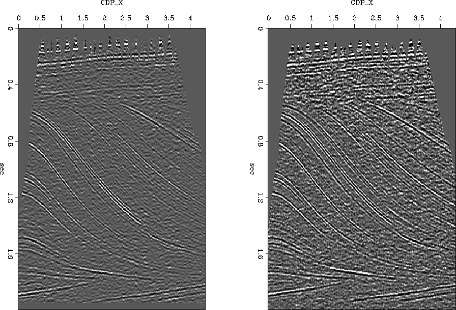
Figure 1 Inline sections through two synthetic datasets. d1 is on the left and d2 is on the right.
Figure 1 shows inline sections through two synthetic surveys, which were created to test 4D seismic processing algorithms. Although they were modeled post-stack, they contain many features derived from actual 4D field datasets, including different wavelets, random noise, spatially varying static and phase shifts, different time-varying gain functions, and different mute and dead-trace zones. The two surveys have different bandwidths and signal-to-noise levels to simulate multi-vintage 3D seismic.
 |
 |
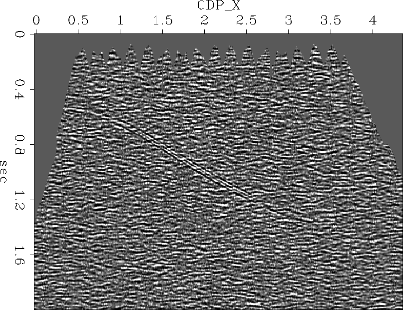
To simulate the effect of production changes, we created base and monitor reflectivity functions by introducing changes along a `reservoir' interval. The best achievable result is shown in Figure 2. This contains only the coherent fluid changes and residual random noise.
A simple cross-equalization flow consists of matched-filtering and amplitude balancing. For this synthetic example, we designed the matched-filters on a trace-to-trace basis, in order to best estimate the spatially-varying static and phase shifts.
Figure 3 shows the filtered survey, ![]() at
the same scale as
at
the same scale as ![]() . The low amplitude of the figure on the
left illustrates the characteristic low value of a due to the noise
in
. The low amplitude of the figure on the
left illustrates the characteristic low value of a due to the noise
in ![]() . The result of the low value of a is coherent
geological signal leaking through into the difference plot, which is
shown in Figure 4. The amplitude of
. The result of the low value of a is coherent
geological signal leaking through into the difference plot, which is
shown in Figure 4. The amplitude of ![]() are equivalent to those obtained by renormalizing the data and scaling
by
are equivalent to those obtained by renormalizing the data and scaling
by ![]() .
.
 |
 |
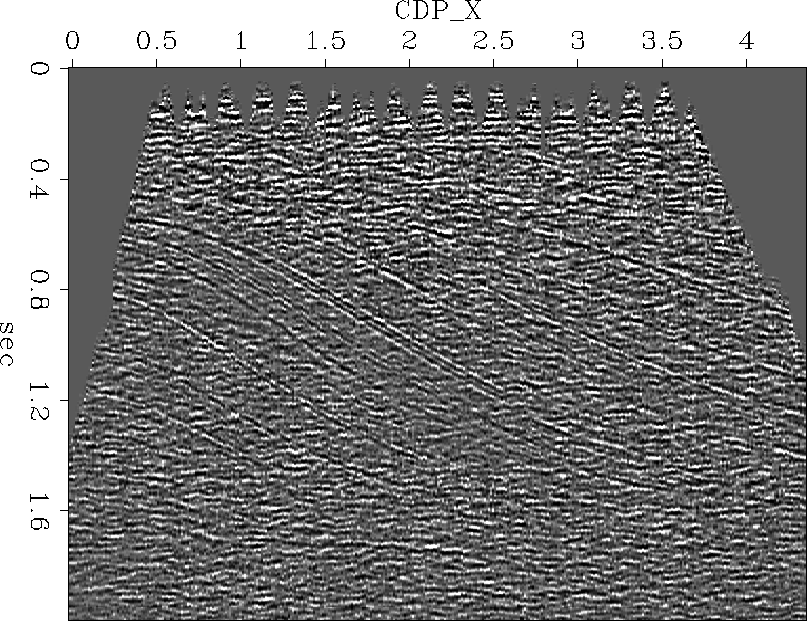
Equalizing the energy in this case (using ![]() ), produces the
poor result shown in Figure 5. The brightest event
in this image is no longer the reservoir interval, but rather the
event below it. This would cause problems for interpretation.
), produces the
poor result shown in Figure 5. The brightest event
in this image is no longer the reservoir interval, but rather the
event below it. This would cause problems for interpretation.
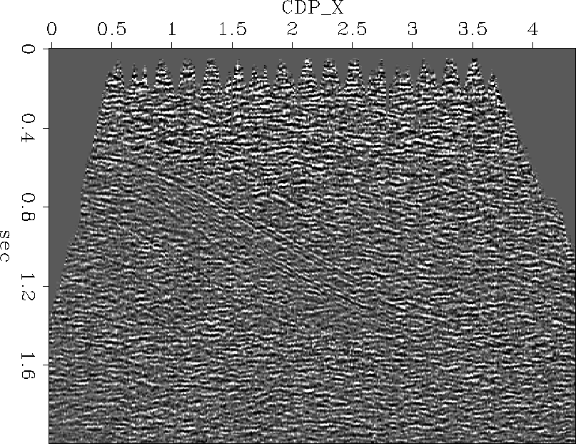
For this synthetic, we can calculate a value for ![]() based on the
known signal-to-noise levels in the two surveys. This gave us the
results shown in Figure 6. Considerably less
coherent energy is present in this image than in
Figures 4 and 5.
based on the
known signal-to-noise levels in the two surveys. This gave us the
results shown in Figure 6. Considerably less
coherent energy is present in this image than in
Figures 4 and 5.
 |
 |