Wavefield composed of two plane waves

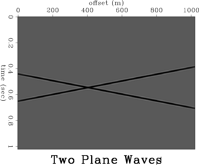
If we have two plane waves, the wavefield (Figure 6) can be expressed by

$$w(t,x) = a_1\delta(t-t_1-p_1x)+a_2\delta(t-t_2-p_2x)$$ (11)

 

two-plane-wave Figure 6 A synthetic wavefield composed of two plane waves.

In the f-x domain, it has another expression

$$W(f,x) = a_1e^{i2\pi f(t_1+p_1x)}+a_2e^{i2\pi f(t_2+p_2x)}$$ (12)

Or

 

W(f,x) = E₁+E₂ (13)

where $E_1 = a_1e^{i2\pi f(t_1+p_1x)}$ and $E_2=a_2e^{i2\pi f(t_2+p_2x)}$.The adjacent trace can be expressed by  

$$W(f,x-\Delta x)=P^{-1}_1E_1+P^{-1}_2E_2$$ (14)

Now we cannot predict one trace from another trace, since there are two unknown propagators. Consequently, we need the information from another trace.  

$$W(f,x-2\Delta x)=P^{-2}_1E_1+P^{-2}_2E_2$$ (15)

Equation (14) and (15) can be solved for the propagators. But in reality, we do not know p₁ and p₂. So we cannot get the explicit form of the propagators. We must use another form of parameter to link the the different traces together, which is called a spatial prediction filter.

If we have trace $x-\Delta x$ and trace $x-2\Delta x$, our aim is to predict trace x. Assume there is a relation between the three traces:

$$W(f,x) = C_1W(f,x-\Delta x)+C_2W(f,x-2\Delta x)$$ (16)

Substituting Ws with equations (13), (14) and (15), we get

 

E₁+E₂ = C₁(P^-1₁E₁+P^-1₂E₂)+C₂(P^-2₁E₁+P^-2₂E₂) (17)

$E_{\rm i}$ can be any value, as long as it is a plane wave. Therefore, equation (17) holds for all of E₁ and E₂. In particular, we have

$$1 = C_1P^{-1}_1+C_2P^{-2}_1, \hspace*{0.2in}(E_1 = 1, \hspace*{0.1in}E_2 = 0)$$ (18)

$$1 = C_1P^{-1}_2+C_2P^{-2}_2, \hspace*{0.2in}(E_1 = 0, \hspace*{0.1in}E_2 = 1)$$ (19)

Solving this linear equation, we find the relation between $C_{\rm i}$ and $P_{\rm i}$ (i=1,2). That is

$$C_1 = P_1 + P_2, \hspace*{0.3in} C_2 = -P_1P_2$$ (20)

Like the one plane wave case, all above deductions have nothing to do with the gridding scheme. All the results are effective for both cases. The differences between the two gridding schemes are

• Frequency-independent grids
  
  As proved before, since the propagator $P_{\rm i}$ depends on frequency, the coefficients of the prediction filter $C_{\rm i}$ will also depend on frequency.
• Frequency-dependent grids
  
  Since the propagator $P_{\rm i}$ is independent of frequency, the coefficients of the prediction filter $C_{\rm i}$ are also independent of frequency.

We can extend our deduction to N plane waves (see the Appendix) and we can get similar results: for FIG, coefficient $C_{\rm i}$ is frequency-dependent; for FDG, $C_{\rm i}$ is frequency-independent. This is the basis of estimating the spatial prediction filter.