Wavefield composed of one plane wave

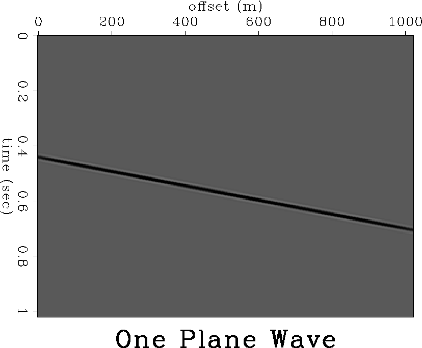
As shown in Figure 5, this wavefield in the t-x domain can be expressed by

$$w(t,x) = \delta (t-t_1-p_1x)$$ (5)

 

one-plane-wave Figure 5 A synthetic wavefield composed of a single plane wave.

After Fourier transform along the time axis, we get the expression in the f-x domain:

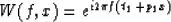$$W(f,x) = e^{i2\pi f (t_1+p_1x)}$$ (6)

It is easy to show that one trace can be predicted from an adjacent trace:

$$W(f,x-\Delta x)=e^{i2\pi f (t_1+p_1x-p_1\Delta x)}=W(f,x)e^{-ip_12\pi f \Delta x}$$ (7)

Or in another form,

$$W(f,x)=e^{ip_12\pi f \Delta x}W(f,x-\Delta x)$$ (8)

This means that, each trace can be predicted with the propagator $P_1=e^{ip_12\pi f \Delta x}$. Up to now, we have not mentioned FIG and FDG. Therefore, all above conclusions are effective for both cases. But when we introduce the details of the two schemes, we will reach different conclusions:

• Frequency-independent grids
  
  $\Delta x = \delta x$ is constant. The propagator P₁ is the function of frequency f. It will change from one frequency slice to another.
• Frequency-dependent grids
  
  From (3), we can choose

  $$\Delta x = \frac{v}{4 f}$$ (9)

  Therefore, the propagator P₁ becomes

  $$P_1 = e^{i\frac{\pi}{2}p_1v}$$ (10)

  So the propagator P₁ is frequency-invariant.