


Next: MODELING REFLECTIONS
Up: REFLECTION AND TRANSMISSION COEFFICIENTS
Previous: Plane wave solutions
At a horizontal interface, we assume a displacement-stress vector whose
variables are continuous across the interface  , where
 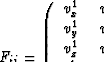 is
the velocity, and
is
the velocity, and  represents the
vertical component of the stress tensor. This vector can be divided
into
represents the
vertical component of the stress tensor. This vector can be divided
into
|  |
(10) |
where the elements of F are
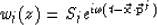
|  |
(11) |
and the elements of the vector  are a function of the wave
amplitudes, as follows:
are a function of the wave
amplitudes, as follows:
|  |
(12) |
To calculate the amplitude partitioning at an interface between two
layers we equate the displacement-stress vector across the interface,
thus:
|  |
(13) |
Translating the coordinate frame so that the interface is at z=0,
the exponential terms in w are the same in both layers, and we can
write equation (13) as
|  |
(14) |
giving a general relation between the up-going and down-going wave
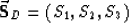
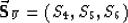
systems in the two media. If we partition  so that
 is a vector of the amplitudes of
down-going waves and
is a vector of the amplitudes of
down-going waves and  of up-going
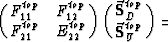
waves, we can write the block-matrix equation as
of up-going
waves, we can write the block-matrix equation as
|  |
(15) |
In order to calculate the up-going reflected wavefield and the
down-going transmitted wavefield for a downward propagating wavefield
incident on the boundary from above, we need to solve the system
|  |
(16) |
After some manipulation, we obtain Nichols (1991)
|  |
(17) |
| |
where
|  |
(18) |
| |
The  matrices RD and TD convert the vector of
down-going wave amplitudes in layer 1 into a vector of up-going
reflected wave amplitudes in layer 1 and a vector of down-going
transmitted amplitudes in layer 2. The next section studies the PP
wave reflection amplitudes given by the first column, first row
element in matrix RD.
matrices RD and TD convert the vector of
down-going wave amplitudes in layer 1 into a vector of up-going
reflected wave amplitudes in layer 1 and a vector of down-going
transmitted amplitudes in layer 2. The next section studies the PP
wave reflection amplitudes given by the first column, first row
element in matrix RD.
Next: MODELING REFLECTIONS
Up: REFLECTION AND TRANSMISSION COEFFICIENTS
Previous: Plane wave solutions
Stanford Exploration Project
11/12/1997