It is important to notice that a point ![]() in data
space fixes the angle
in data
space fixes the angle ![]() of the incident plane wave as well. Because
of the Bragg condition, the
of the incident plane wave as well. Because
of the Bragg condition, the ![]() dependence in model space is transformed
into incidence-angle dependence, according to
dependence in model space is transformed
into incidence-angle dependence, according to
 |
(4) |
For each point in the (kx, kz) domain, that is for each
sinusoidal component in the space domain,
the ![]() dependence is a vector
dependence is a vector
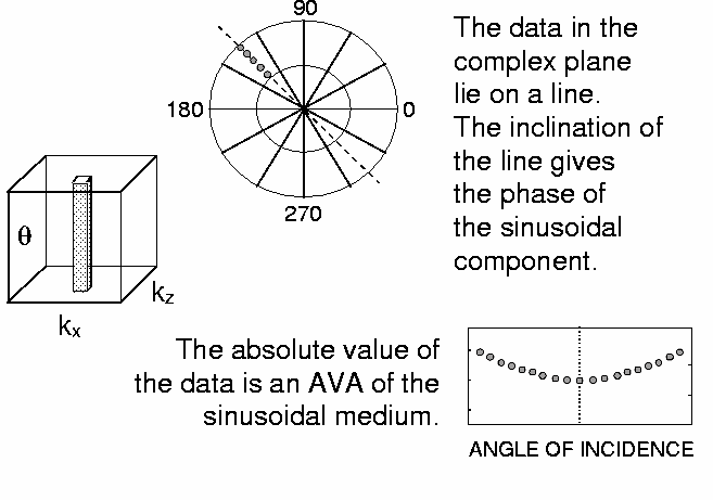
![]() . This represents the Phase versus Angle (PvA)
and Amplitude versus Angle (AvA) of the sinusoidal component of the
medium (Figure 4),
. This represents the Phase versus Angle (PvA)
and Amplitude versus Angle (AvA) of the sinusoidal component of the
medium (Figure 4),
| |
(5) |
with
![]()
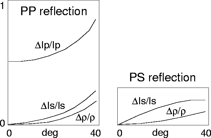
The matrix G describes the reflection angle dependence, the wavelet spectrum, the propagation effects and the directivity of sources and receivers. Figure (5) illustrates the reflection coefficient of a sinusoidal medium due to unitary parameter perturbations for P-P and P-SV reflections.
 |
|
unitary
Figure 5 Theoretical AvA of a sinusoidal medium for a unitary change of parameters. |  |
The inversion is a least-squares fit of the measured PvA and AvA,
which is the result of the mapping process,
with the theoretical PvA and AvA in the complex plane.
We use the SVD decomposition of the relation data-parameters
![]() (Lines and Treitel 1984).
The matrix
(Lines and Treitel 1984).
The matrix ![]() contains the eigenvectors in data space.
contains the eigenvectors in data space.
![]() is the diagonal matrix of singular values.
They represent the energy in the data due to a unitary
variation along eigenvectors axis in the model space.
is the diagonal matrix of singular values.
They represent the energy in the data due to a unitary
variation along eigenvectors axis in the model space.
![]() contains the eigenvectors in model space: they form an
orthogonal basis in the model space and are linear
combinations of the elastic parameters perturbations
contains the eigenvectors in model space: they form an
orthogonal basis in the model space and are linear
combinations of the elastic parameters perturbations
![]() ,
, ![]() and
and ![]() .
.
The reflections of each sinusoidal component are inverted one
by one: given (kx, kz) and the corresponding migrated data
![]() ,
,
| |
(6) |
The data ![]() , plotted in the complex plane, form a line
(Figure 4).
The inclination of the line gives the phase of the sinusoidal component.
The absolute value of the data is the measured AvA of the sinusoidal medium.
, plotted in the complex plane, form a line
(Figure 4).
The inclination of the line gives the phase of the sinusoidal component.
The absolute value of the data is the measured AvA of the sinusoidal medium.
Because of the finite range of sources, receivers, frequency components and observation angles, only a part of the entire model spectrum can be recovered. Non-observable components of the spectrum (null space) are not inverted. Sharp transitions of the angular coverage in the (kx, kz) domain are tapered before transformation to the x-z panels.
The ill-conditioning of the inverse elastic problem can lead, because of the presence of numerical inaccuracies and interpolation errors, to interference between parameters estimates. De Nicolao et al. (1993) have found that with realistic signal-to-noise-ratios, in this linearized approach, P-P reflections allow an accurate estimation of P-impedance perturbation only. S-impedance perturbation can be recovered with multicomponent data, namely P-SV reflections. Density perturbations are practically unrecoverable. We have tested these results on synthetic examples, which are described below.