


We follow the procedure outlined by Bernasconi et al. (1994).
P-wave isotropic point sources and receivers are located on the
surface of a medium characterized by small 2D deviations of the
elastic parameters from a known uniform background.
We compute synthetic seismograms using the linearized scatter
patterns of a point diffractor (Wu and Aki, 1985) and the Born approximation:
small reflection coefficients make multiple reflections negligible.
The reflectivity is expressed as a linear combination of elastic perturbations.
The chosen parameter set is P-impedance relative perturbations
![]() , S-impedance relative perturbations
, S-impedance relative perturbations ![]() and
density relative perturbations
and
density relative perturbations ![]() .The input data is a set of common shot gathers.
They form a cube (data space) whose axes are
.The input data is a set of common shot gathers.
They form a cube (data space) whose axes are
A Fourier transformation over source and offset coordinate leads to a cube in the domain
Transformation to the ![]() domain (model domain) is
accomplished through diffraction tomography techniques (Wu and Toksö, 1987).
To illustrate the basic principle of diffraction tomography we
consider an infinite medium and an incident monochromatic
plane wave with wavenumber
domain (model domain) is
accomplished through diffraction tomography techniques (Wu and Toksö, 1987).
To illustrate the basic principle of diffraction tomography we
consider an infinite medium and an incident monochromatic
plane wave with wavenumber ![]() .
The reflected plane wave
.
The reflected plane wave ![]() depends upon only one Fourier
component of the medium (Figure 1).
depends upon only one Fourier
component of the medium (Figure 1).
Let ![]() be the vector of medium wavenumbers (kx, kz).
The relation between the medium wavenumber and the incident and
reflected waves is
be the vector of medium wavenumbers (kx, kz).
The relation between the medium wavenumber and the incident and
reflected waves is
| |
(1) |
A reflected plane wave due to an incident plane wave illuminates only one
point in the model space (kx, kz):
this is a Bragg resonance effect.
Therefore the mapping of data space (t, ks, kh) into the model space
![]() is
is
| kx = ks, | (2) |
| |
(3) |
where vr and vi are the velocities of the reflected and incident waves, respectively.
|
diff-tomog
Figure 1 Diffraction Tomography: the Bragg effect. A reflected and an incident monochromatic plane wave enlighten only one sinusoidal component of the medium. | 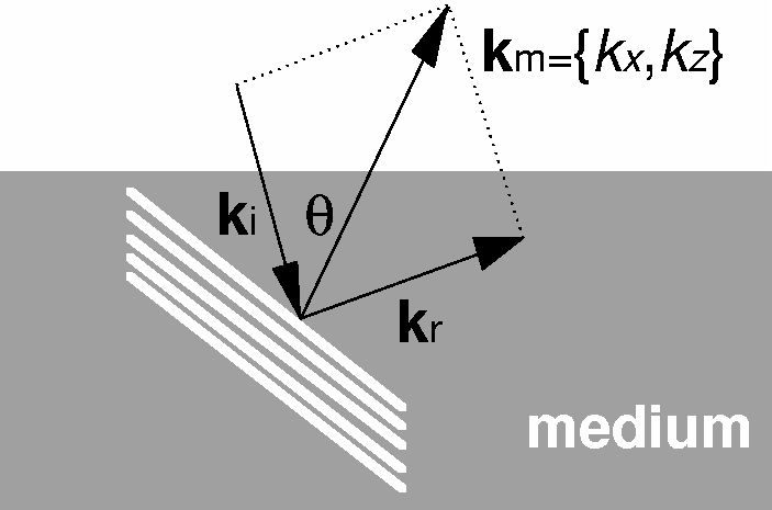 |

Given kx and kz, we solve equations
(2) and (3) to obtain a value of ![]() for each value
of kh. The data are migrated through a t-
for each value
of kh. The data are migrated through a t-![]() transform.
The t-
transform.
The t-![]() transform is evaluated with a DFT.
This operation is performed one point at a time in the (kx,kz) domain,
so we collect the contributions to the reflected
field of a single sinusoidal perturbations at a time.
transform is evaluated with a DFT.
This operation is performed one point at a time in the (kx,kz) domain,
so we collect the contributions to the reflected
field of a single sinusoidal perturbations at a time.
Spectral coverage is affected by cable length (angular aperture) and finite bandwidth. With surface acquisition, the horizontal wavenumbers are not recoverable (Figures 2 and 3) as they fall in the non-observable part of the spectrum (null space).
|
kxkz-domain
Figure 2 Coverage of the model spectrum with surface acquisition and limited bandwidth from | 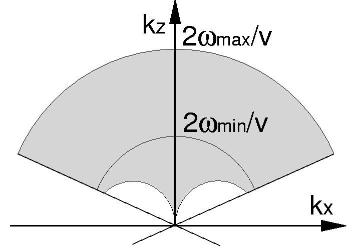 |
|
mod-spec
Figure 3 Effects of the limited angular aperture and bandwidth on the spectrum and on the model. Horizontal variations in the model are unrecoverable with surface acquisition as they fall in the non-observable part of the spectrum. | 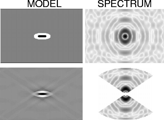 |