Editing in two-dimensional data

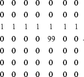
Two-dimensional data provides a more challenging problem, but also a more useful one. Consider the following as an example of two-dimensional data with noise:  

$$\begin{array} {ccccccc} 0 & 0 & 0 & 0 & 0 & 0 & 0 \\ 0 & 0 &... ...& 0 & 0 & 0 & 0 & 0 \\ 0 & 0 & 0 & 0 & 0 & 0 & 0 \end{array}.$$ (10)

Assume that the vertical axis of () corresponds to the time axis, and that the horizontal axis corresponds to the space axis. This dataset has a horizontal event plus a noise spike. An obvious method of removing the noise is to apply the one-dimensional filter () to either the rows or the columns of (). Applying filter () to the rows would be making the assumption that reflection events are flat. This approach would be valid for the dataset in () since the signal is flat. Applying filter () to the columns, or along the time axis, would generally not be valid, since reflections are assumed to be unpredictable, and predictable events within a trace indicate undesirable noise.

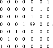
For a dataset such as  

$$\begin{array} {ccccccc} 0 & 0 & 0 & 0 & 0 & 0 & 1 \\ 0 & 0 &... ...& 0 & 0 & 0 & 0 & 0 \\ 1 & 0 & 0 & 0 & 0 & 0 & 0 \end{array},$$ (11)

two-dimensional filters are needed to predict the sloping event. One such filter is  

$$\begin{array} {cc} 0 & -1 \\ 1 & 0 \\ 0 & 0\end{array}.$$ (12)

In the case of real seismic data, the filters are computed from the data. While the filters could be calculated over several traces, I limit the prediction of a trace to include only its immediate neighbors. These filters have the form  

$$\begin{array} {cc} 0 & a_{1} \\ 0 & a_{2} \\ 1 & a_{3} \\ 0 & a_{4} \\ 0 & a_{5} \end{array}$$ (13)

to predict a trace from the right, and the form  

$$\begin{array} {cc} b_{1} & 0 \\ b_{2} & 0 \\ b_{3} & 1 \\ b_{4} & 0 \\ b_{5} & 0 \end{array}$$ (14)

to predict a trace from the left. In these filters, the output point is under the 1 coefficient. The vertical axis of this filter is time, the bs cover the trace used for the prediction, and the column with the single 1 coefficient covers the trace being predicted. Both these filters are calculated as annihilation filters as described in chapter , so that if the trace is well predicted, the residual will be almost zero. A small residual indicates that the trace is dominated by signal.

Two filter calculations are done for each trace, one for each filter shown above. When these filters are applied, two sets of residuals are created. These two sets of residuals are combined into a single set of residuals by taking a sample-by-sample minimum of the absolute values of the two residuals. This single residual is then used as the diagnostic for noise. The single residual allows a sample to be predicted from either the right or from the left by taking the best of the two original predictions.

Once the set of minima of the absolute values of the residuals is created, the median of all the minima within a window is calculated. Although measures other than the median, such as the RMS of a window, could be used, the median is likely to provide a better diagnostic of a typical value within a window. Zero values are ignored when calculating the median, so that traces that were not present or muted on the input to the process do not contribute to the value of the median. Any value greater than w times the median value calculated is considered to be caused by high-amplitude noise. The value of w is determined by examining the data processed with a range of ws. In the examples shown here, a w of five was used, although the process seems to be somewhat insensitive to the exact values of w, as can be seen with Figure  in the electronic version of this thesis. Samples in the original data are eliminated when the corresponding values in the single residual are greater than w times the median within a window. A flowchart describing the entire process is shown in figure .

 

flowchart Figure 1 A flowchart of the sample deletion process.