


Instead of using nearest neighbor interpolation in space I now use linear interpolation in space. The value at every point on the path is linearly interpolated from the two neighboring traces.
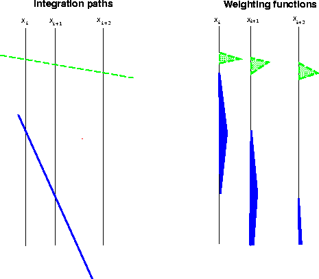 |

Figure ![[*]](http://sepwww.stanford.edu/latex2html/cross_ref_motif.gif) shows the region of the traces used in this method. The
trace is used from the point at which the trajectory crosses the previous trace
to that at which it crosses the next trace. At each point on the curve
the value is linearly interpolated from the two surrounding traces. So that
shows the region of the traces used in this method. The
trace is used from the point at which the trajectory crosses the previous trace
to that at which it crosses the next trace. At each point on the curve
the value is linearly interpolated from the two surrounding traces. So that
![]()
The weighting function is a triangle. It has its peak at the point that the trajectory crosses the trace, and it has an area equal to the average distance to the neighbor traces. If the integral were a time integral, the limits of the triangle would be the same but it would have a unit peak height.
This method is closely related to the second method described by Claerbout, in which he uses triangular weights in Kirchoff migration.