


Before considering interpolation in both space and time I will first consider two cases where only interpolation in space is required. In these methods the traces are assumed to be continuous functions of time.
![]()
The first method uses nearest neighbor interpolation in space.
The value at every point on the curve is taken from the nearest
trace.Figure ![[*]](http://sepwww.stanford.edu/latex2html/cross_ref_motif.gif) shows the values interpolated at every point on
the trajectory. As the trajectory gets steeper a greater length of
each trace is used in the integral. The trace is used from the time
at which the trajectory crosses (xix + xix-1)/2 to the time
at which it crosses (xix+1+xix)/2. The function
shows the values interpolated at every point on
the trajectory. As the trajectory gets steeper a greater length of
each trace is used in the integral. The trace is used from the time
at which the trajectory crosses (xix + xix-1)/2 to the time
at which it crosses (xix+1+xix)/2. The function
![]() is the function through which the line integral is
actually calculated. If this is a good approximation to the true function
the the integral will be close to the true integral.
is the function through which the line integral is
actually calculated. If this is a good approximation to the true function
the the integral will be close to the true integral.
![]()
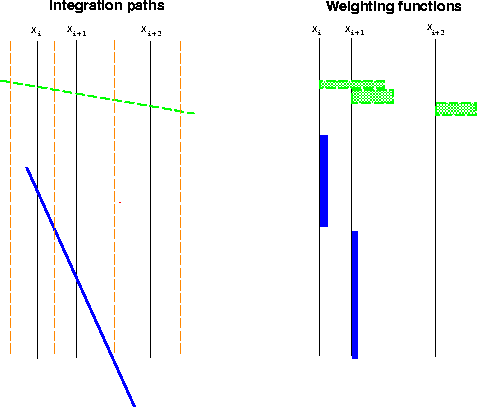 |

The weighting function on each trace is a rectangle of area equal to the average distance to the neighbor traces, note that this is because our integral is cast as an integral in x; if it were an integral in t, the rectangles would all be of unit height.
This method is closely related to the first method described by Claerbout, 1992 where a rectangular weights are used to perform an anti-aliased Kirchoff migration.