The finite difference algorithm described by Van Trier and Symes (1991) is based on the eikonal equation in cartesian coordinates
| u2+v2=s2 | (1) |

| |
(2) |

The traveltime is propagated one depth step at a time in cartesian coordinates, or
one radial step at a time in cylindrical coordinates. The values of ![]() and
and ![]() are calculated
on each computational front. The domain of dependence is given by the length ratio
of the two vectors
are calculated
on each computational front. The domain of dependence is given by the length ratio
of the two vectors ![]() and
and ![]() , as seen in Figure 1.
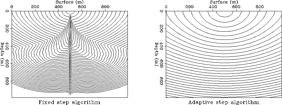
The fixed grid algorithm is faster than the adaptive algorithm, sometimes by
a factor of 10-20, depending on the velocity model considered.
However numerical instabilities like the one in Figure 2 can not be predicted.
The slower adaptive step algorithm will offer robust results.
, as seen in Figure 1.
The fixed grid algorithm is faster than the adaptive algorithm, sometimes by
a factor of 10-20, depending on the velocity model considered.
However numerical instabilities like the one in Figure 2 can not be predicted.
The slower adaptive step algorithm will offer robust results.
 |
My initial adaptive step calculation in polar coordinates, based on the geometrical arguments presented in Figure 1, is listed below.
The calculations are done for each new radial computational front. The variable ddr is the initial radial increment which is modified adaptively. The arrays v and u store the values of the functions defined in equation (2). The minimum angle for the domain of dependence is calculated for each computational front and the minimum radial increment is used to advance the front.
A more elegant approach was suggested by Dave Hale. It
monitors the same domain of dependence condition avoiding all the
time consuming trigonometric relations. It also avoids the
division by zero that can occur in either the case of u=0
or v=0.
Essentially, the trick is to check for the ratio between v and
![]() in the form
in the form v * r <= TINY * u which
increases the dynamic range of the variables compared.