HORIZONTALLY LAYERED INVERSION

While equation (4) is linear in t² for the homogeneous case, the introduction of layers disrupts this linearity because here we must add traveltimes and not traveltimes squared. This non-linearity represents a problem if the model space is composed of layers (or cells), because the excessive number of unknowns brings not only a prohibitive cost, but also an increasing degree of instability in the solution as the number of model parameters increase. One possible solution is to linearize the problem, and solve it in an iterative scheme. Another is to decompose the model into an orthogonal set of functions and solve for each component independently.

I use here an approach that is closely related to this second form, but which substantially simplifies the forward computations in the initial iterations. Moreover, because of the way it builds the solution- by the introduction of successive degrees of complexity, this method is highly stable.

Similarly to the Fourier decomposition, the method represents the sloth model as composed by the superposition of two sets of oscillatory functions (one set comprised of symmetric functions and the other comprised of anti-symmetric functions), plus a constant factor that accounts for the average-model  

$${\bf M} = c + \sum_{i=1}^N a_i \: {\cal S}_i + \sum_{i=1}^N b_i \: {\cal C}_i.$$ (5)

The basis functions ${\cal S}_i$ and ${\cal C}_i$ are sine-like and cosine-like square waves with an integer number of cycles i, with a fixed length corresponds to the total depth interval spanned by the model. I will not address here the discussion about the orthogonality and completeness of the basis set of functions and the space spanned by them, but rather emphasize their practicality as model generators in the inversion scheme that follows.

The first step of the method corresponds to the homogeneous inversion described in the previous section, and it accounts for the component c in equation (5). Next, an iterative process is applied, in which the ith iteration corresponds to a perturbation in the solution of the previous iteration; the perturbation is formed by a linear combination of the two basis functions of order i (that is, i cycles). Figure  shows how the perturbations in the model are constructed for the first two iterations. As explained in the figure caption, the actual parameters to be estimated at each iteration are not a and b, but dM₁ and dM₂, which are directly related to the perturbations in each layer. Since we must consider perturbations in M^x as well as in M^z, the number of independent parameters to be estimated at each iteration will always be four: dM^x₁, dM^x₂, dM^z₁, and dM^z₂.

Differently from the Fourier decomposition, here the number of points (layers) describing the model is not fixed for the retrieval of all the frequency components, but instead increases proportionally to the sequential number of the iteration. At each iteration, the total number of layers is four times the sequential number of the iteration. The solution is constructed in successive degrees of resolution, which results in a highly stable method, despite the use of a non-linear optimization algorithm.

The objective function to be minimized at each iteration is  

$${\cal F} = \sum_{i=1}^N \sum_{j=J_i}^{L_i} \left( t_{ij} - t^{\prime}_{ij} \right)^2,$$ (6)

where N is the number of shots, J_i and L_i refer to the extreme receivers of shot number i, t_ij is the measured traveltime corresponding to shot i and receiver j, and $t^{\prime}_{ij}$is the traveltime predicted by the perturbed model. Using the straight-rays approximation, the predicted traveltime is given by

$$\begin{eqnarray} t^{\prime}_{ij} & = & \sum_{k=K_i}^{K_j} {o}_k \sqrt{(M^x_k + {... ..._k + {s}_k dM^x_2) x_{ijk}^2 + (M^z_k + {s}_k dM^z_2) z_{ijk}^2},\end{eqnarray}$$ (7)

where o_k, e_k, and s_k are defined as  

$${o}_k = {1-(- \! 1)^k \over 2}, \mbox{\hspace{2.0cm}} {e}_k... ... \over 2}, \mbox{\hspace{2.0cm}} {s}_k = (- \! 1)^{(k+3) / 2}.$$ (8)

In equation (7) the subscript k is the number of a particular layer (for this particular iteration), while K_i and K_j correspond to the layers where the source i and receiver j are localized respectively. The horizontal x_ijk and the vertical z_ijk distances traveled by the ray that links source i to receiver j inside the layer k are constants for all but the first and last layers.

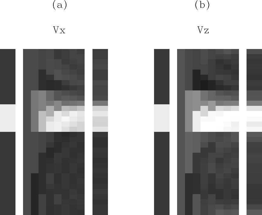
I applied the method to a synthetic dataset corresponding to a single isotropic horizontal layer immersed in an also isotropic background. The data consists of traveltimes from 20 shots localized in one well, each recorded by 51 receivers localized in the other well. The space between adjacent sources was 5 times as larger as the distance between adjacent receivers. The layer thickness and the distance between wells were 3.33 and 3.6 times the distance between sources, respectively. Figure 1 shows the original and the retrieved models, as well as the partial result of each iteration.

The final results for V_x and V_z are close enough to the original model, if we consider the resolution limit associated with the specific acquisition-parameters and geometry. As expected, the part of the model that corresponds to V_x converges faster, and for a better solution, than the part that corresponds to V_z. The layer thickness in the last iteration is about 3/5 the source interval.

 

hetmod
Figure 1 Original synthetic model and successive results of the layered inversion scheme. (a) Is the V_x part of the model, while (b) is the V-z part. In both cases the extreme left column is the original model and the extreme right is the result of the 8th iteration (32 layers); they are displayed with a vertical exaggeration of 1.5 relative to the actual dimensions. The intermediary columns correspond to the results of the homogeneous inversion and all the successive iterations (1-7). They are displayed with half the horizontal width of the extremes for purposes of compactness.