Residual moveout-based wave-equation migration velocity analysis in 3-D

3-D transforms between offset and angle domain

Our RMO-based WEMVA approach operate exclusively on subsurface angle domain CIGs, however, compared to ADCIGs, subsurface offset domain CIGs are much friendlier for computer implementation. The image-space tomographic operator on ODCIGs also has a simpler formula and can be straightforwardly implemented (Tang et al., 2008). Therefore transforming between ODCIGs and ADCIGs is required for our approach. Tisserant and Biondi (2003) and Biondi and Tisserant (2004) presented the theory for this tranformation. We review the key steps in the offset to angle transformation:

1. Perform Fourier transform $I(hx,hy,x,y,z) \rightarrow I(hx,hy,k_x,k_y,k_z)$ .
2. For each $(k_x,k_y,k_z)$ ,
   • apply Fourier transform $I(hx,hy) \rightarrow I(k_{hx},k_{hy})$
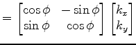
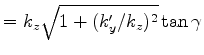
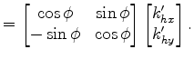
   • map $I(k_{hx},k_{hy}) \rightarrow I(\gamma,\phi)$ based on the following relations (Tisserant and Biondi, 2003):

     $$\begin{bmatrix}k'_{x} \\ k'_{y} \end{bmatrix} = \begin{bmatrix}\cos\phi & -\sin\phi \\ \sin\phi & \cos\phi \end{bmatrix} \begin{bmatrix}k_x \\ k_y \end{bmatrix}$$

     $$k'_{hx} = {k_z} \sqrt{1+(k'_y/k_z)^2} \tan\gamma$$

     $$k'_{hy} = \frac{k'_y k'_x k'_{hx}}{k^{'2}_y + k_z^2}$$

     $$\begin{bmatrix}k_{hy} \\ k_{hy} \end{bmatrix} = \begin{bmatrix}\cos\phi & \sin\phi \\ -\sin\phi & \cos\phi \end{bmatrix} \begin{bmatrix}k'_{hx} \\ k'_{hy} \end{bmatrix}.$$ (21)

     
     

3. Apply inverse Fourier transform $I(\gamma,\phi,k_x,k_y,k_z) \rightarrow I(\gamma,\phi,x,y,z)$ .

Similarly, the backward transform (angle to offset) is done by reversing the order of the procedures above.

a2omapping0,a2omapping1
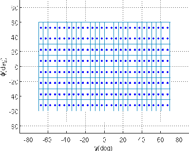
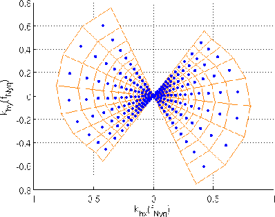
Figure 4. Graphical illustration of the mapping from the $(\gamma ,\phi )$ plane to the $(k_{hx},k_{hy})$ plane. Each dot in (a) maps to a corresponding dot in (b); similarly, each quadrilateral patch in (a) maps to a corresponding patch in (b).

The mapping between $(\gamma ,\phi )$    and $(k_{hx},k_{hy})$ is highly irregular (Biondi, 2003). Figure 4 shows the mapping from a regularly sampled $(\gamma ,\phi )$ mesh to the $(k_{hx},k_{hy})$ domain given fixed $k_z = 1/2,\; k_x = 1/4$    and $k_y = 1/4$ (assume the Nyquist wave number is 1). We can see the mapping brings distortion, and the density of the samples on $(k_{hx},k_{hy})$ becomes non-uniform. A proper interpolation scheme is very important to reduce the artifacts caused by such irregularity. This issue becomes more serious for the backward transform (angle to offset), because the azimuth angle $\phi$ is usually not sufficiently sampled; simply placing all available samples on the $(\gamma ,\phi )$ plane onto their mapped locations on $(k_{hx},k_{hy})$ plane would leave many holes unfilled. On the other hand, under mapping relation 21, it is easy to map from a given $(\gamma ,\phi )$ value to $(k_{hx},k_{hy})$ , but it is difficult to do the reverse due to the algebra. Therefore, it is very difficult to iterate over all points on $(k_{hx},k_{hy})$ , find the corresponding $(\gamma ,\phi )$ coordinates, and fetch the values on these coordinates.

We choose a simple yet effective scheme to perform this mapping. Instead of mapping from sample points to sample points (dots in Figure 4), we map from quadrilateral patches to quadrilateral patches, assuming each patch contains uniformly the value of the sample located in its center. We use a classic polygon-filling algorithm for this mapping. After that, a slight amount of smoothing is applied on the output to remove potential discontinuities along the boundaries of the patches.

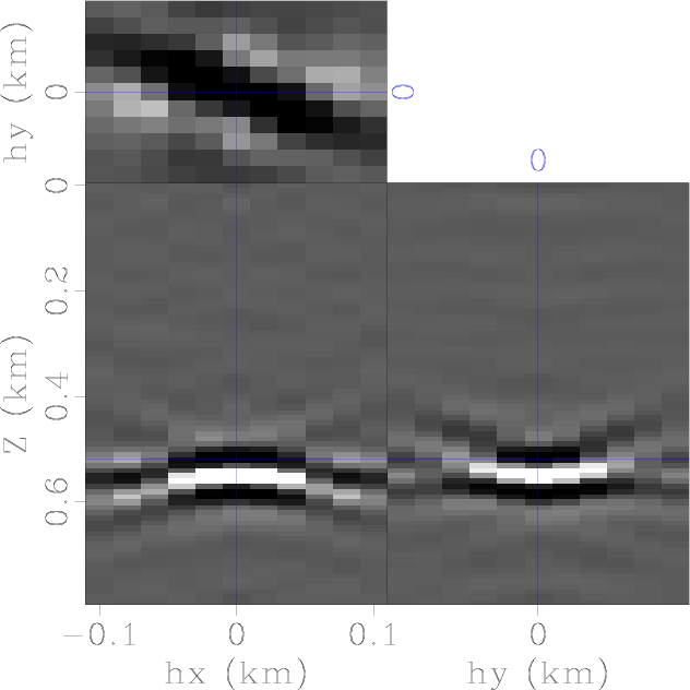
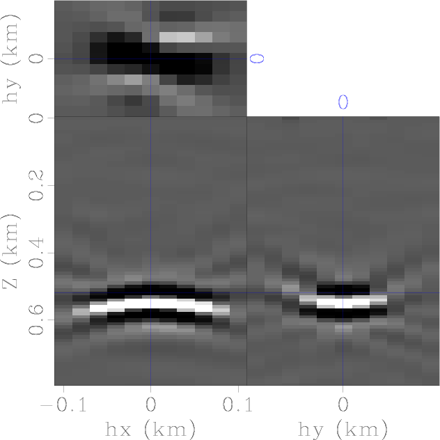
We use the previous synthetic example to demonstrate the necessity of this scheme. We start with an initial subsurface ODCIG by migrating the data using the starting velocity model, as shown in Figure 5(c). Then we apply our forward and backward offset-angle transforms to the ODCIG sequentially (Figure 5(b)). For comparison, we also compute the result using the transform that simply does sample-to-sample mapping (Figure 5(a)). A good transform pair should make the resulting ODCIG resemble the original one as closely as possible. Notice there is no way we can retrieve a result exactly same as the original gather, because the information in azimuth range 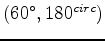$(60^{\circ},180^{circ})$ is lost in the angle domain CIG. Nonetheless, it is obvious that Figure 5(b) is less distorted than Figure 5(a) is. Our mapping scheme would reduce the artificial noise that arises during the transform of image perturbation from angle back to offset domain.

offNN,offPF,offori
Figure 5. (a) The result of applying forward and backward offset-angle domain transform on an ODCIG, in which the sample-to-sample mapping is used; (b) the same description as (a), except that the patch-to-patch mapping is used. The original ODCIG is shown in (c). All three gathers are chosen at location $x=0.2\ensuremath{\, \mathrm{km}}, y=-0.06\ensuremath{\, \mathrm{km}}$ . Notice that the intermediate ADCIG we generate does not have full azimuth coverage ( $[60^{\circ },180^{\circ }]$ excluded), therefore an exactly identical reconstruction of the original ODCIG is not possible.

Residual moveout-based wave-equation migration velocity analysis in 3-D