Implicit finite difference in time-space domain with the helix transform

Validity tests of derived coefficients

Before implementing the methodology discussed above, I tested whether the finite-difference weights derived in Equation 10 for the implicit approximation are indeed reversible by a set of convolution and deconvolution operators. The input impulse used for the tests is shown in Figure 4. The sequence of operations applied to this impulse were:

1. forward deconvolution with the spectrally factorized coefficients of the above finite-difference weights.
2. adjoint deconvolution.
3. adjoint convolution.
4. forward convolution.

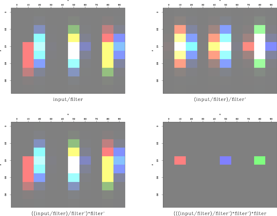
The sequence and it's results are shown in Figure 5. The final result is not a perfect impulse, however the remaining values in the wavefield are 6 or more orders of magnitude smaller than the central impulse.

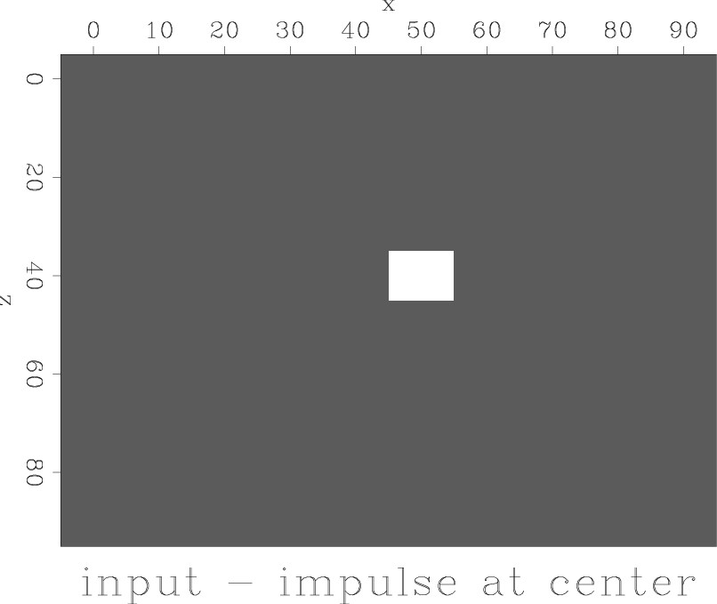
imp-test3-in Figure 4. Input impulse used for helical convolution test

imp-test3-panels Figure 5. Results of convolving and deconvolving with filter coefficients whose convolution yields the finite-difference weights required by the implicit finite-difference approximation in Equation 17

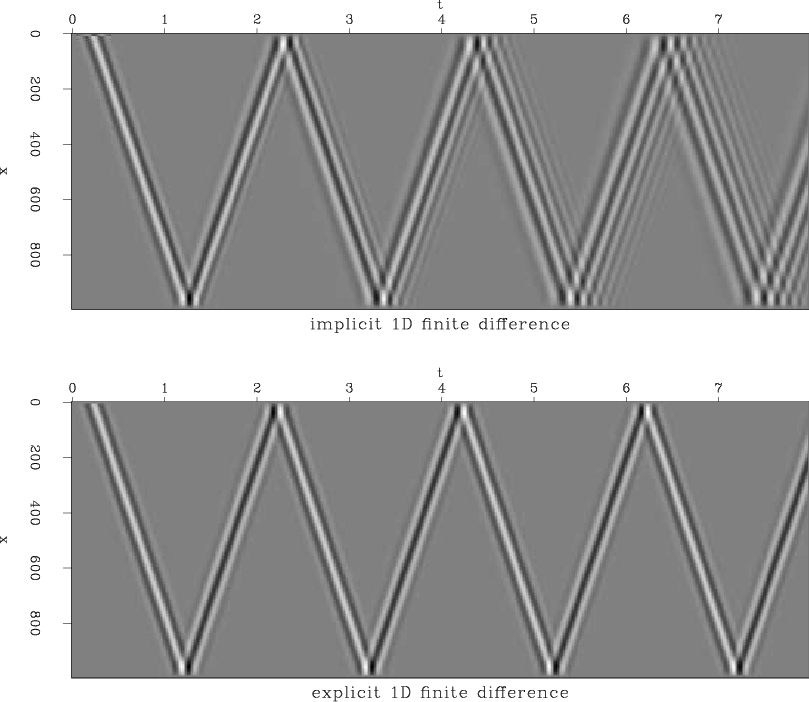
exp-vs-imp-1d
Figure 6. 1D Explicit Vs. Implicit finite difference with constant velocity = $1000 m/s$ . Source is a Ricker wavelet with central frequency = $12.5 Hz$ . The explicit time step was $\Delta t = 4 msec$ . The implicit time step was $\Delta t = 8 msec$ . $\Delta x = 10 m$ .

In order to test whether the derived implicit finite-difference coefficients are actually valid for wavefield propagation, the next step was to compare standard explicit finite difference to implicit propagation with these coefficients in one dimension. The implicit solution was done using the SEPlib module rtris which recursively solves a tridiagonal equation system. The results are in Figure 6. Severe dispersion is visible in the implicitly propagated wavefield. So far I have been unable to remove this dispersion without damaging the kinematics of the wavefield.
On the other hand, the wavefield derived by implicit finite difference does not diverge even when increasing the temporal time step beyond the stability limit of the explicit solver.

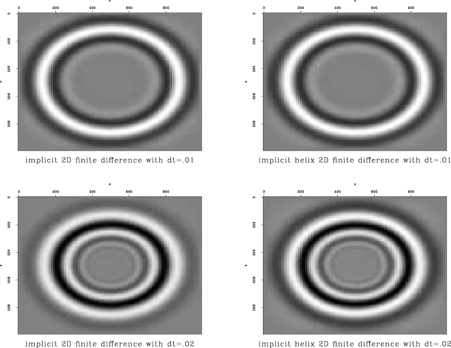
imp-vs-helimp-snap
Figure 7. 2D Implicit Vs. Helical Implicit finite difference with constant velocity = $1000 m/s$ . Source is a Ricker wavelet with central frequency = $12.5 Hz$ . The time step for the top figures was $\Delta t = 10 msec$ , and for the bottom figures $\Delta t = 20 msec$ . $\Delta x = \Delta z = 10 m$ .

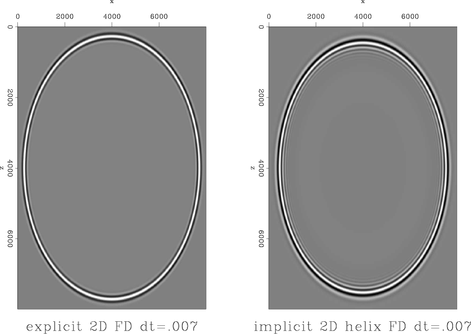
exp-vs-helimp-snap
Figure 8. 2D Explicit Vs. Helical Implicit finite difference with constant velocity = $1000 m/s$ . Source is a Ricker wavelet with central frequency = $12.5 Hz$ . The time step was $\Delta t = 7 msec$ - at the stability limit of the explicit scheme for the 2nd order in time and space approximation. $\Delta x = \Delta z = 10 m$ .

Implicit finite difference in time-space domain with the helix transform