Formulation for 2 dimensions

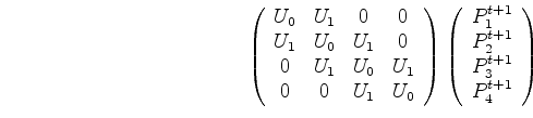
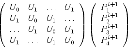
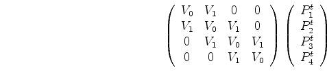
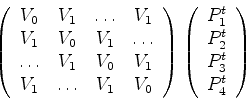
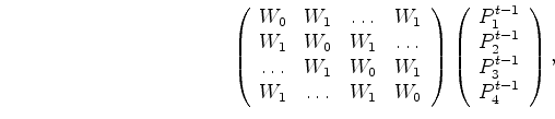
The finite-difference weights for the 2-D case of matrix

(where $\Delta x = \Delta z$ ) are derived by using the same finite-difference approximation (2nd order in time and space) as in Equation 9. The derived linear equation system is similar to the one shown in (10), except that two off-diagonal bands appear at a certain offset from the main diagonal. The offset is equal to the number of elements of the ``fast'' axis of the 2D wavefield.

$\begin{displaymath}\left( \begin{array}{ccccc} U_0 & U_1 & \dots & U_1 \\ U_1 &... ..._1 \\ P^{t+1}_2 \\ P^{t+1}_3 \\ P^{t+1}_4 \end{array}\right)\end{displaymath}$	$\displaystyle =$	$\begin{displaymath}\left( \begin{array}{ccccc} V_0 & V_1 & \dots & V_1 \\ V_1 &... ...rray}{c} P^t_1 \\ P^t_2 \\ P^t_3 \\ P^t_4 \end{array}\right)\end{displaymath}$
	$\displaystyle +$	$\begin{displaymath}\left( \begin{array}{ccccc} W_0 & W_1 & \dots & W_1 \\ W_1 &... ...1 \\ P^{t-1}_2 \\ P^{t-1}_3 \\ P^{t-1}_4 \end{array}\right),\end{displaymath}$	(17)

where the finite-difference weights are:
$U_0 = 1 + 4 \alpha, U_1 = -\alpha;$
$V_0 = 2 - 4 \alpha, V_1 = \alpha;$
$W_0 = -1 - 4 \alpha, W_1 = \alpha,$
and where $\alpha = \frac{C^2 \Delta t^2}{3 \Delta x^2}.$

The propagation methodology is the same as shown in Equation 14 - creation of a solution vector, and then two deconvolutions using the SEPlib polydiv module.

The main advantage in comparison to a standard linear equation system solver is in the reduced number of operations required to propagate the wavefield by one time step. The computation time scales linearly with the size of the data and the number of factorized filter coefficients, instead of the square of the size of the data. Coupled with the larger time steps which are made possible by an implicit finite-difference scheme, this methodology has the potential to reduce total processing times for wavefield propagation algorithms. The further advantage is the separation of the solution from the dimensionality of the problem.