|
|
|
|
Implicit finite difference in time-space domain with the helix transform |
For simplicity, we can combine all the constants into one:
 .
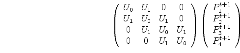
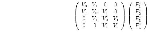
The matrix coefficients in Equation 10 (the finite-difference weights) are then:
.
The matrix coefficients in Equation 10 (the finite-difference weights) are then:
![]()
![]()
![]()
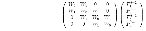
In shorter notation, Equation 10 reads:
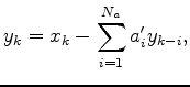
The solution of this linear system is:
To solve this system, we must perform polynomial division. The system is tridiagonal (and easily solvable) only for 1 dimension. For multiple dimensions, matrix ![]() is block diagonal. Additional non-zero elements appear at a certain offset from the diagonal, making the solution process more complicated. However, using spectral factorization, the finite-difference weights of matrix
is block diagonal. Additional non-zero elements appear at a certain offset from the diagonal, making the solution process more complicated. However, using spectral factorization, the finite-difference weights of matrix ![]() can be factorized into a set of causal filter coefficients
can be factorized into a set of causal filter coefficients ![]() and it's time reverse
and it's time reverse ![]() . Using the helical approach to deconvolution, the system can be recast as:
. Using the helical approach to deconvolution, the system can be recast as:
As stated above, polynomial division is equal to deconvolution. This means that the polynomial division in Equation 12 can be achieved by a set of two deconvolutions of the spectrally factorized coefficients ![]() of matrix
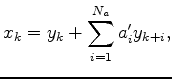
of matrix ![]() . One deconvolution is done along the data in the reverse direction (application of the adjoint of the filter):
. One deconvolution is done along the data in the reverse direction (application of the adjoint of the filter):
 is the time reversed filter coefficients of
I used the SEPlib module polydiv, which uses the helical coordinates to do the deconvolutions (the polynomial division) in equations 15 and 16.
The wavefield propogation is done by the following sequence:
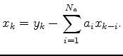 .
.
This sequence is repeated for each time step.
|
|
|
|
Implicit finite difference in time-space domain with the helix transform |