Wave-equation tomography for anisotropic parameters

Inversion for 2-D VTI models

From the gradient given by the anisotropic WETom operator in last section, we notice that the perturbations in slowness and $\eta$ are co-located. This is an intrinsic characteristic of the operator, which may not be geologically realistic. Therefore, we design three tests to examine this effect in the inversion.

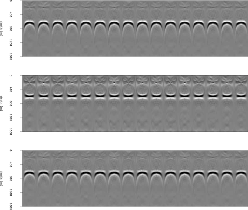
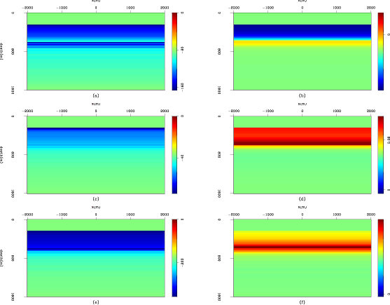
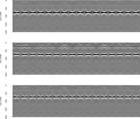
In these three tests, we use the same initial model (Figure 5), but data modeled using different true models. In Figure 6 we show the true model perturbations, which have one layer of perturbations in slowness only, in $\eta$ only, and in both. Figure 7 shows the angle-domain common image gathers (ADCIGs) using the initial model, where ADCIGs are not flat due to the error in the model. Notice the image perturbation is small for the perturbation in $\eta$ only.

In the inversion, we define the focusing operator in the perturbed image (Equation 7) by the Differential Semblance Optimization (DSO) method (Shen, 2004):

$${\bf F}({\bf I}) = ( {\bf 1} - {\bf O}){\bf I},$$ (21)

where ${\bf 1}$ is the identity operator and ${\bf O}$ is the DSO operator. Therefore, the objective function (Equation 8) becomes:

$$J = \frac{1}{2}\vert\vert{\bf O \widehat{\bf I}}\vert\vert^2 = \frac{1}{2}\vert\vert h {\bf\widehat{\bf I}}\vert\vert^2,$$ (22)

where $h$ is the subsurface half-offset. Since the DSO operator is independent of the model parameters, the gradient of $J$ with respect to the model parameters is

$${\bf\nabla} J = \left.\left(\frac{\partial {\bf I}}{\partial {\bf... ...st}{\bf O}\widehat{\bf I} = {\bf T}^{\ast}{\bf O}^{\ast}{\bf O}\widehat{\bf I}.$$ (23)

To minimize the objective function, we specifically use the steepest descent algorithm. To help convergence, we average the gradient at each depth to ensure a layered model and mute the shallow updates to avoid near-surface artifacts.

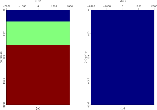
init
Figure 5. Initial model for inversion. Panel (a) is the initial velocity model with three layers; Panel (b) is the initial $\eta$ model with constant value of zero.

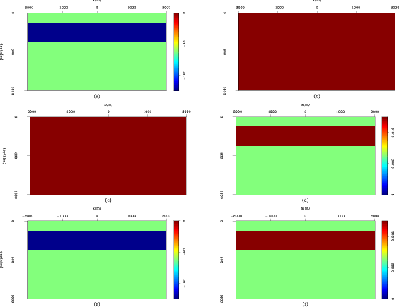
truep
Figure 6. True model perturbation in three test cases. Panel (a) and (b): Perturbation in velocity only; Panel (c) and Panel (d): Perturbation in $\eta$ only; Panel (e) and Panel (f): Perturbations in both.

initimage
Figure 7. ADCIGs using the initial model in three cases. Top panel: Perturbation in velocity only; Middle panel: Perturbation in $\eta$ only; Bottom panel: Perturbations in both. Curvature in the ADCIGs indicates errors in velocity or $\eta$ .

update
Figure 8. Inversion results of the three test cases. Panels are comparable to those in Figure 6.

finalimage
Figure 9. Common image gathers using the updated model in three cases. Top panel: Perturbation in velocity only; Middle panel: Perturbation in $\eta$ only; Bottom panel: Perturbations in both. ADCIGs are flattened compared with Figure 7.

Figure 8 shows the final model updates after 4 non-linear iterations. The results should be comparable to the model perturbations in Figure 6. In the final updates, we see a consistent over predition of $\eta$ . This is because error in $\eta$ has a very smal contribution in the image perturbation, as shown in the middle panel of Figure 7. Figure 9 shows the ADCIGs using the updated model. Comparing Figure 6 and Figure 8, Figure 7 with Figure 9, we can conclude that the inversion successfully identifies the layered perturbation and flattens the ADCIGs. However, back-projection of the residual image shows up in both parameter spaces, although it is caused by perturbations in a single parameter. Also for the case of perturbing both spaces, the over-prediction of velocity perturbation and the under-prediction of $\eta$ perturbation reconcile with each other and produce flat events in the ADCIGs. Therefore, we can conclude that the ambiguity between the velocity and the anellipticity cannot be resolved simply by the inversion, and auxiliary information is needed to further distinguish the difference.

Wave-equation tomography for anisotropic parameters