|
|
|
|
Wave-equation tomography for anisotropic parameters |
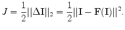
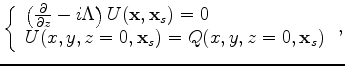
In the least-squares sense, the tomographic objective function can be written as follows:
To perform the WETom for anisotropic parameters, we first need to
extend the tomographic operator from the isotropic medium
(Shen, 2004; Sava, 2004; Guerra et al., 2009) to the anisotropic medium. We
define the image-space wave-equation tomographic operator T for anisotropic
parameters as follows:
 |
|||
 |
(9) |
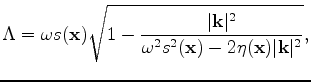
 and anellipticity parameter
 | (10) |
Both source and receiver wavefields are downward continued in the shot-profile
domain using the one-way wave equations (Claerbout, 1971):
 is the source wavefield at the image
point
is the source wavefield at the image
point
 is the angular frequency,
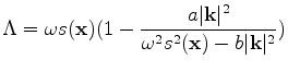 . Using
binomial expansion, Equation 14 can be further expanded
to polynomials:
. Using
binomial expansion, Equation 14 can be further expanded
to polynomials:
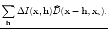
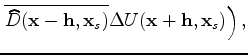
The background image is computed by applying the cross-correlation
imaging condition:
 is the subsurface half-offset.
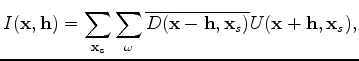
Under the Born approximation, a perturbation in the model parameters
causes a first-order perturbation in the wavefields. Consequently, the
resulting image perturbation reads:
 and
and
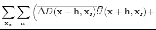
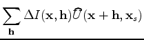
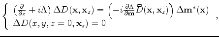
To evaluate the adjoint tomographic operator
![]() , which
backprojects the image perturbation into the model space, we first
compute the wavefield perturbation from the image perturbation using
the adjoint imaging condition:
, which
backprojects the image perturbation into the model space, we first
compute the wavefield perturbation from the image perturbation using
the adjoint imaging condition:
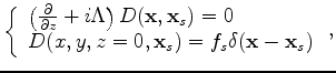
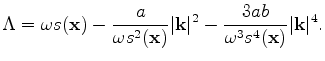
The perturbed source and receiver wavefields satisfy the following
one-way wave equations, linearized with respect to slowness and ![]() :
:
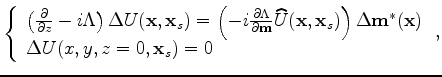 is the row vector
.
is the row vector
.
When solving the optimization problem, we obtain the image perturbation by migrating the data with the current background model and performing a focusing operation (Equation 7). Then the perturbed image is convolved with the background wavefields to get the perturbed wavefields (Equation 18). The scattered wavefields are computed by applying the adjoint of the one-way wave-equations 19 and 20. Finally, the model space gradient is obtained by cross-correlating the upward propagated scattered wavefields with the modified background wavefields (terms in the parentheses on the right-hand sides of Equations 19 and 20).
|
|
|
|
Wave-equation tomography for anisotropic parameters |