Wave-equation tomography for anisotropic parameters

Numerical test of the anisotropic WETom operator

To test the anisotropic WETom operator, we run the forward and adjoint WETom operator on a 2-D model. Figure 1 shows the background isotropic model, with one reflector in velocity and no anisotropy. The data are modeled with 4000m maximum offset, 8m receiver spacing, 80m source spacing and 41 split-spread shots. We use the two-way acoustic anisotropic modeling code in Madagascar to do the modeling, and the one-way SSF (Tang and Clapp, 2006) extrapolator to do the migration.

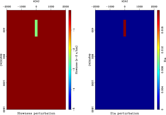
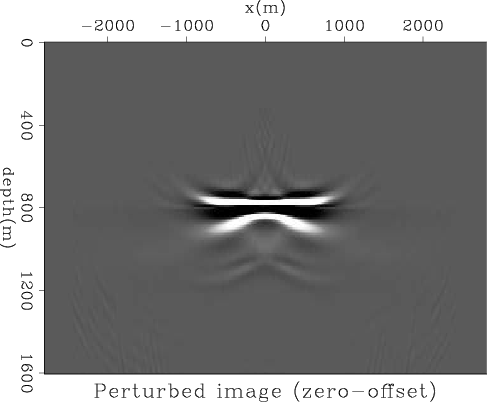
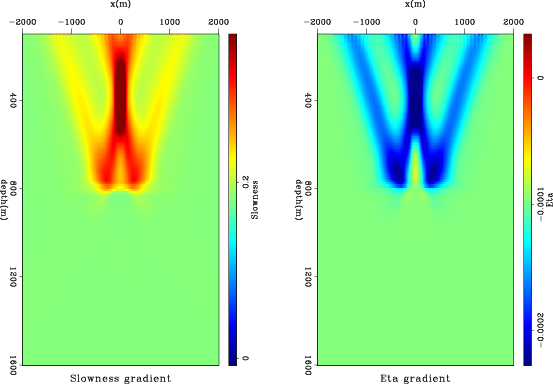
Figure 2 shows the model perturbations, with a rectangular slowness anomaly that is 10% lower than the background slowness on the left, and a rectangular anisotropic anomaly on the right. The perturbation in $\eta$ within the rectangular block is constant ( $\Delta \eta = 0.1$ ). Figure 3 shows the perturbed image at the zero lag of the subsurface offset due to the model perturbations after applying the forward WETom operator. Adjoint WETom operator back-projects the perturbed image into the model space, and outputs the gradient for the model perturbation, as shown in Figure 4. Comparing Figure 2 and Figure 4, we can see that the gradients provide the correct direction and shape of the perturbation to conduct a line search in a given inversion scheme.

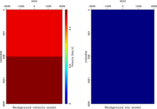
background
Figure 1. Background isotropic model. Left is the velocity model with one reflector, and right is the $\eta$ model with constant zero.

perturb
Figure 2. Model perturbations. Left is a rectangular slowness anomaly that is 10% lower than the background slowness , and right is a rectangular anisotropic anomaly with a constant value of $\Delta \eta = 0.1$ .

Dimage Figure 3. Perturbed image from the forward anisotropic WETom operator. The image is extracted from the zero lag of the subsurface offset.

Dmodel
Figure 4. Back-resolved gradient for the model updates. Left is the gradient for slowness, and right is the gradient for $\eta$ .

Wave-equation tomography for anisotropic parameters