Blocky models via the L1/L2 hybrid norm

Non-linear solver

The non-linear approach is a little more complicated but it explicitly deals with the interaction between $\bf s$ and $\bf c$ so it converges faster. We represent everything as a ``known'' part plus a perturbation part which we will find and add into the known part. This is most easily expressed in the Fourier domain.

$$0 \quad \approx\quad (S + \Delta S) (C+\Delta C) - D$$ (37)

Linearize by dropping $\Delta S \Delta C$.

$$0 \quad \approx\quad S \Delta C +  C \Delta S + (CS -D)$$ (38)

Let us change to the time domain with a matrix notation. Put the unknowns $\Delta C$ and $\Delta S$ in vectors $\tilde{\bf c}$ and $\tilde{\bf s}$. Put the knowns $C$ and $S$ in convolution matrices $\bf C$ and $\bf S$. Express $CS-D$ as a column vector $\bar {\bf d}$. Its time domain coefficients are $d_0=c_0 s_0 - d_0$ and $d_1=c_0 s_1 + c_1 s_0 -d_1$, etc. The data fitting regression is now

$$\bf0 \quad \approx \quad {\bf S} \tilde{\bf c} + {\bf C} \tilde{\bf s} + \bar{\bf {d}}$$ (39)

This regression is expressed more explicitly below.

$$\bf0 \quad \approx \quad \left[ \begin{array}{cccccccccc} s_0& . ... ...d_0 \ d_1 \ d_2 \ d_3 \ d_4 \ d_5 \ d_6 \ d_7 \ d_8 \end{array} \right]$$ (40)

The model styling regression is simply $0\approx C + \Delta C$, which in familiar matrix form is

$$\bf0 \quad\approx\quad \bf I  \tilde{\bf c} + \bar {\bf c}$$ (41)

It is this regression, along with a composite norm and its associated threshold that makes $c(t)$ come out sparse. Now we have the danger that $\bf c\rightarrow 0$ while $\bf s\rightarrow \infty$ so we need one more regression

$$\bf0 \quad\approx\quad \bf I  \tilde{\bf s} + \bar {\bf s}$$ (42)

We can use ordinary least squares on the data fitting regression and the shot waveform regression. Thus

$$\bf0 \quad\approx\quad \left[ \begin{array}{c} \bf r_d \ \bf r_s \end{array}\right] = \left[ \begin{array}{cc} \bar {\bf S} &\bar {\bf C} \\ {\bf0... ...\begin{array}{c} \bar {\bf d}\ \bar {\bf s} \end{array}\right]$$ (43)

$$\bf0 \quad\approx\quad \bf r = \bf F \bf m + \bf d$$ (44)

The model styling regression is where we seek spiky behavior.

$$\bf0 \quad\approx\quad \bf r_c = \bf I  \tilde{\bf c} + \bar{\bf c}$$ (45)

The big picture is that we minimize the sum

$$\min_{\tilde{\bf c},\tilde{\bf s}} \quad N_d(\bf r) + \epsilon N_m(\bf r_c)$$ (46)

Inside the big picture we have updating steps

$$\Delta\bf m = \bf F' \bf r$$ (47)

$$\bf g_d = \Delta\bf r = \bf F \Delta \bf m$$ (48)

We also have a gradient for changing $\tilde{\bf c}$, namely $\bf g_c = - \bar {\bf c}$. (I need to be sure $\bf g_d$ and $\bf g_c$ are commensurate. Maybe need an $\epsilon$ here.) One update step is to choose a line search for $\alpha$

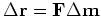
$$\min_\alpha \quad N_d( \bf r + \alpha \bf g_d) +  \epsilon N_m(\bar{\bf c} + \alpha \bf g_c)$$ (49)

That was steepest descent. The extension to conjugate direction is straightforward.

As with all nonlinear problems there is the danger of bizarre behavior and multiple minima. To avoid frustration, while learning you should spend about half of your effort directed toward finding a good starting solution. This normally amounts to defining and solving one or two linear problems. In this application we might get our starting solution for $s(t)$ and $c(t)$ from conventional deconvolution analysis, or we might get it from the block cyclic solver.

Blocky models via the L1/L2 hybrid norm