 |
 |
 |
 | Blocky models via the L1/L2 hybrid norm |  |
![[pdf]](icons/pdf.png) |
Next: Non-linear solver
Up: UNKNOWN SHOT WAVEFORM
Previous: UNKNOWN SHOT WAVEFORM
In the Block Cyclic solver (I hope this is the correct term.), we have two half cycles.
In the first half we take one of the variables known and the other unknown. We solve for the unknown.
In the next half we switch the known for the unknown.
The beauty of this approach is that each half cycle is a linear problem
so its solution is independent of the starting location. Hooray!
Even better, repeating the cycles enough times should converge to the correct solution. Hooray again!
The convergence may be slow, however,
so at some stage (maybe just one or two cycles) you can safely switch over to the nonlinear method
which converges faster because it deals directly with the interactions of the two variables.
We could begin from the assumption that the shot waveform is an impulse and the reflectivity is the data.
Then either half cycle can be the starting point.
Suppose we assume we know the reflectivity,
say  , and solve for the shot waveform
  .
We use the reflectivity to make a convolution matrix
.
We use the reflectivity to make a convolution matrix  .
The regression pair for finding is
.
The regression pair for finding is
These would be solved for by familiar least squares methods.
It's a very easy problem because has many fewer components than .
Now with our source estimate
we can define the operator  that convolves it on reflectivity .
The second half of the cycle is to solve for the reflectivity .
This is a little trickier.
The data fitting may still be done by an  type method,
but we need something like an
type method,
but we need something like an  method for the regularization
to pull the small values closer to zero to yield a more spiky
method for the regularization
to pull the small values closer to zero to yield a more spiky  .
.
Normally we expect an
 in equation (31) but now it comes in later.
(It might seem that the regularization (29) is not necessary,
but without it, might get smaller and smaller while gets larger and larger.
We should be able to neglect regression (29) if we simply rescale appropriately at each iteration.)
We can take the usual L2 norm
to define a gradient vector for model perturbation
in equation (31) but now it comes in later.
(It might seem that the regularization (29) is not necessary,
but without it, might get smaller and smaller while gets larger and larger.
We should be able to neglect regression (29) if we simply rescale appropriately at each iteration.)
We can take the usual L2 norm
to define a gradient vector for model perturbation
 .
From it we get the residual perturbation
.
From it we get the residual perturbation
 .
We need to find an unknown distance
.
We need to find an unknown distance 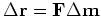 to move in those directions.
We take the norm of the data fitting residual,
add to it a bit
to move in those directions.
We take the norm of the data fitting residual,
add to it a bit  of the model styling residual,
and set the derivative to zero.
of the model styling residual,
and set the derivative to zero.
![$\displaystyle \bold 0 \quad=\quad \frac{\partial}{\partial\alpha} [ N_d(\bold...
...\alpha \; \Delta\bold r ) + \epsilon N_m(\bold c + \alpha \Delta \bold c ) ]$](img120.png) |
(32) |
We need derivatives of each norm at each residual.
We base these on the convex function  of the Hybrid norm.
Let us call these
of the Hybrid norm.
Let us call these 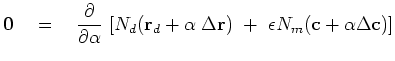 for the data fitting,
and
for the data fitting,
and  for the model styling.
(Actually, we don't need
(because for Least Squares,  and
and  ),
but I include it here in case we wish to deal with noise bursts in the data.)
As earlier, expanding the norms in Taylor series,
equation (32) becomes
),
but I include it here in case we wish to deal with noise bursts in the data.)
As earlier, expanding the norms in Taylor series,
equation (32) becomes
 |
(35) |
which gives the we need to update the model and the residual 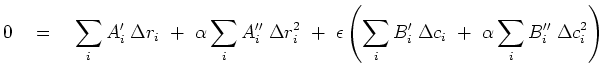 .
.
 |
(36) |
This is the steepest descent method.
For the conjugate directions method
there is a 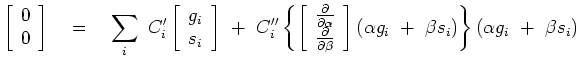 equation like
equation (24).
equation like
equation (24).
|
|
|
|
| Blocky models via the L1/L2 hybrid norm | |
|
Next: Non-linear solver
Up: UNKNOWN SHOT WAVEFORM
Previous: UNKNOWN SHOT WAVEFORM
2009-10-19