Blocky models via the L1/L2 hybrid norm

PLANE SEARCH

The most universally used method of solving immense linear regressions such as imaging problems is the Conjugate Gradient (CG) method. It has the remarkable property that in the presence of exact arithmetic, the exact solution is found in a finite number of iterations. A simpler method with the same property is the Conjugate Direction method. It is debatable which has the better numerical roundoff properties, so we generally use the Conjugate Direction method as it is simpler to comprehend. It says not to move along the gradient direction line, but somewhere in the plane of the gradient and the previous step. The best move in that plane requires us to find two scalars, one $\alpha$ to scale the gradient, the other $\beta$ to scale the previous step. That is all for $L2$ optimization. We proceed here in the same way with other norms and hope for the best.

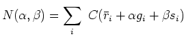
So here we are, embedded in a giant multivariate regression where we have a bivariate regression (two unknowns). From the multivarate regression we are given three vectors in data space. $\bar r_i$, $g_i$ and $s_i$. You will recognize these as the current residual, the gradient ( $\Delta r_i$), and the previous step. (The gradient and previous step appearing here have previously been transformed to data space (the conjugate space) by the operator $\bold F$.) Our next residual will be a perturbation of the old one.

$$r_i \quad=\quad \bar r_i + \alpha g_i + \beta s_i$$ (20)

We seek to minimize by variation of $(\alpha,\beta)$

$$N(\alpha,\beta) = \sum_i C (\bar r_i+\alpha g_i +\beta s_i)$$ (21)

Let the coefficients $(C_i,C_i',C_i'')$ refer to a Taylor expansion of $C(r)$ about $r_i$.

$$N(\alpha,\beta)= \sum_i C_i + (\alpha g_i +\beta s_i)C_i' + (\alpha g_i +\beta s_i)^2 C_i''/2$$ (22)

We have two unknowns, $(\alpha,\beta)$ in a quadratic form. We set to zero the $\alpha$ derivative of the quadratic form, likewise the $\beta$ derivative getting

$$\left[ \begin{array}{c} 0 \ 0 \end{array} \right] \quad=\quad \s... ...array} \right] (\alpha g_i + \beta s_i) \right\} (\alpha g_i + \beta s_i)$$ (23)

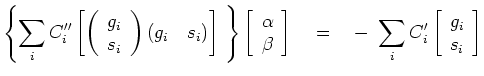
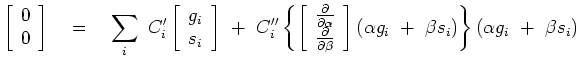resulting in a $2\times 2$ set of equations to solve for $\alpha$ and $\beta$.

$$\left\{ \sum_i C_i'' \left[ \left( \begin{array}{c} g_i \ s_i\en... ...quad=\quad - \sum_i C_i' \left[ \begin{array}{c} g_i \ s_i\end{array} \right]$$ (24)

The solution of any $2\times 2$ set of simultaneous equations is generally trivial. The only difficulties arise when the determinant vanishes which here is easy (luckily) to understand. Generally the gradient should not point in the direction of the previous step if the previous move went the proper distance. Hence the determinant should not vanish. Practice shows that the determinant will vanish when all the inputs are zero, and it may vanish if you do so many iterations that you should have stopped already, in other words when the gradient and previous step are both tending to zero.

Using the newly found $(\alpha,\beta)$, update the residual $\bar r_i$ at each location (and update the model). Then go back to re-evaluate $C_i'$ and $C_i''$ at the new $r_i$ locations. Iterate.

In what way do we hope/expect this new bivariate solver embedded in a conjugate direction solver to perform better than old IRLS solvers? After paying the inevitable price, a substantial price, of computing $\bold F'\bold r$ and $\bold F\; \Delta \bold m$ the iteration above does some serious thinking, not a simple linearization, before paying the price again.

If the convex function $C(r)$ were least squares, subsequent iterations would do nothing. Although the Taylor series of the second iteration would expand about different residuals $r_i$ than the first iteration, the new second order Taylor series are the exact representation of the least squares penalty function, i.e. the same as the first - so the next iteration goes nowhere.

Will this computational method work (converge fast enough) in the $L1$ limit? I don't know. Perhaps we'll do better to approach that limit (if we actually want that limit) via gradually decreasing the threshold $R$.

Blocky models via the L1/L2 hybrid norm