Poroelastic measurements resulting in complete data sets for granular and other anisotropic porous media

Inverting poroelastic compliance

The matrix in (22) is in compliance form and has extremely simple poroelastic behavior in the sense that all the fluid mechanical effects appear only in the single coefficient $\gamma$. I can simplify the notation a little more by lumping some coefficients together, combining the $3\times3$ submatrix in the upper left corner of the matrix in (22) as ${\bf S}$, and defining the column vector ${\bf b}$ by

$${\bf b}^T \equiv (\beta_1, \beta_2, \beta_3).$$ (37)

The resulting $4\times4$ matrix and its inverse are now related by:

$$\left(\begin{array}{cc} {\bf S} & -{\bf b} \cr -{\bf b}^T & \gamm... ...(\begin{array}{cc} {\bf A} & {\bf q} \cr {\bf q}^T & z\end{array} \right)^{-1},$$ (38)

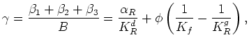
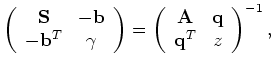where the elements of the inverse matrix can be shown to be written in terms of drained stiffness matrix ${\bf C}^d = {\bf C} = {\bf S}^{-1}$ by introducing three components: (a) scalar $z = \left[\gamma - {\bf b}^T{\bf C}{\bf b}\right]^{-1}$, (b) column vector ${\bf q} = z{\bf C}{\bf b}$, and (c) undrained $3\times3$ stiffness matrix (i.e., the pertinent one connecting the principal strains to principal stresses) ${\bf A} = {\bf C} + z{\bf C}{\bf bb}^T{\bf C} = {\bf C}^d + z^{-1}{\bf qq}^T \equiv {\bf C}^u$, since ${\bf C}^d$ is drained stiffness and ${\bf A} = {\bf C}^u$ is clearly undrained stiffness by construction. This result is the same as that of Gassmann (1951) for anisotropic porous media, although his results were presented in a form somewhat harder to scan than the form shown here.

Also, note the important fact that the observed decoupling of the fluid effects occurs only in the compliance form (22) of the equations, and never in the stiffness (inverse) form for the poroelasticity equations.

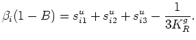
From these results, it is not hard to show that

$${\bf S}^d = {\bf S}^u + \gamma^{-1}{\bf bb}^T.$$ (39)

This result emphasizes the remarkably simple fact that the drained compliance matrix can be found directly from knowledge of the inverse of undrained compliance, and the still unknown, but sometimes relatively easy to estimate, values of $\gamma$, together with the three distinct orthotropic $\beta_i$ coefficients, for $i = 1,2,3$.

renewedcommandarraystretch1.2 par begincenter sc Table 1. Reuss (R), Voigt (V), and self-consistent effective ($*$) bulk moduli of various common anisotropic materials cite[]berryman05: Water ice, cadmium, zinc, graphite, $alpha$-quartz, corundum, barium titanate, rutile, aluminum, copper, magnesia, spinel. Full references for the data used in both sc Tables 1 and 2 are provided in citeberryman05. Units of bulk modulus $K$ are GPa.

par begintabular|c|c|c|c|c|c| hlinehline Material & Symmetry & $K_R$ & $K^*$ & $K_V$ & $K_V/K_R$ 
hline H$_2$O & Hexagonal &   8.89 &   8.89 &   8.89  & 1.00 
Cd & Hexagonal &  48.8  &  54.7  &  58.1   & 1.19 
Zn & Hexagonal &  61.6  &  70.9  &  75.1   & 1.22 
 Graphite  & Hexagonal  &  35.8  &  88.0   & 286.3   & 8.00 
hline Al$_2$O$_3$ & Trigonal & 253.5  & 253.7  & 253.9   & 1.002
$alpha$-SiO$_2$ & Trigonal &  37.6  &  37.8  &  38.1   & 1.01 
hline TiO$_2$ & Tetragonal & 209   & 213   & 218    & 1.04 
BaTiO$_2$ & Tetragonal & 163.1  & 179.3 & 186.8   & 1.15 
hline Al & Cubic &  76.3  &  76.3 &  76.3   & 1.00 
MgO & Cubic & 162.4  & 162.4  & 162.4   & 1.00 
MgAl$_2$O$_4$ & Cubic & 196.7  & 196.7  & 196.7   & 1.00 
Cu & Cubic & 138.0  & 138.0  & 138.0   & 1.00 
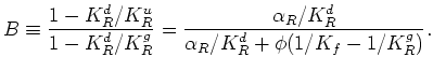
hlinehline endtabular endcenter par subsectionDeducing coefficients from measurements: Anisotropic example with homogeneous grains par Now, further progress is made by considering the Reuss average again for both of the orthotropic drained and undrained compliances: beginequation frac1K_R^d equiv sum_i,j = 1,2,3 s^d_ij, labeleq:drainedKR endequation and beginequation frac1K_R^u equiv sum_i,j = 1,2,3 s^u_ij. labeleq:undrainedKR endequation These effective moduli are the Reuss averages of the nine compliances in the upper left $3\times3$ of the full (including the uncoupled shear components) $6times6$ compliance matrix for the two cases, respectively, when the pore fluid is allowed to drain from the porous system, and when the pore fluid is trapped by a jacketing material and therefore undrained. par 1.2

TABLE 2.(R), Voigt (V), and self-consistent effective ($*$) shear moduli of various common materials [see Berryman (2005)]: Water ice, cadmium, zinc, graphite, $alpha$-quartz, corundum, barium titanate, rutile, aluminum, copper, magnesia, and spinel. Units of shear modulus $G$ are GPa. The anisotropy parameter ${\cal A}$ $\equiv 5\frac{G_V}{G_R} + \frac{K_V}{K_R} - 6$ [from Ranganathan and Ostoja-Starzewski (2008a,b)].

Material	Symmetry	$G_R$	$G^*$	$G_V$	$G_V/G_R$	${\cal A}$
H$_2$O	Hexagonal	3.48	3.52	3.55	1.02	0.10
Cd	Hexagonal	22.1	24.3	26.4	1.19	1.14
Zn	Hexagonal	34.1	40.6	44.8	1.31	1.77
Graphite	Hexagonal	9.2	52.6	219.4	23.8	121.0
Al$_2$O$_3$	Trigonal	160.7	163.1	165.5	1.03	0.15
$alpha$-SiO$_2$	Trigonal	41.0	44.0	47.6	1.16	0.81
TiO$_2$	Tetragonal	99.5	114.5	124.9	1.26	1.34
BaTiO$_2$	Tetragonal	47.4	53.6	59.8	1.26	1.46
Al	Cubic	26.0	26.2	26.3	1.01	0.05
MgO	Cubic	123.9	126.3	128.6	1.04	0.20
MgAl$_2$O$_4$	Cubic	98.6	109.0	118.0	1.20	1.00
Cu	Cubic	40.0	46.3	51.3	1.28	1.41

Although the significance of the formula in the anisotropic case is somewhat different now, I find again that

$$\beta_1+\beta_2+\beta_3 = \frac{1}{K_R^d} - \frac{1}{K_R^g} = \frac{\alpha_R}{K_R^d},$$ (40)

if I also define a Reuss effective stress coefficient:

$$\alpha_R \equiv 1 - K_R^d/K_R^g,$$ (41)

by analogy to the isotropic case. Furthermore, I have

$$\gamma = \frac{\beta_1+\beta_2+\beta_3}{B} = \frac{\alpha_R}{K_R^d} + \phi\left(\frac{1}{K_f} - \frac{1}{K_R^g}\right),$$ (42)

since I have the rigorous result in this notation (Berryman, 1997) that Skempton's $B$ coefficient (Skempton, 1954) is given by

$$B \equiv \frac{1-K_R^d/K_R^u}{1-K_R^d/K_R^g} = \frac{\alpha_R/K_R^d}{\alpha_R/K_R^d + \phi(1/K_f - 1/K_R^g)}.$$ (43)

I want to emphasize that all these formulas are rigorous statements based on the earlier anisotropic analysis. The appearance of $K_R^d$ and $\alpha_R$ is not an approximation. In fact it is important now in the anisotropic case (but not in the isotropic cases considered earlier as long as the grains were also homogeneous) to make this distinction between the Reuss and Voigt averages. Making this choice of notation will help demonstrate useful analogies between the rigorous anisotropic formulas and the isotropic ones. I have prepared the way for these analogies by using the Reuss averages in earlier notation, even though they were mostly redundant in those isotropic examples.

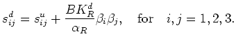
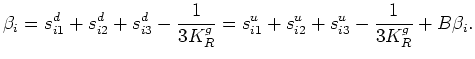
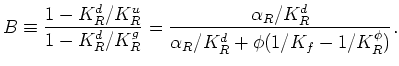
First note that, from (42) and (44), it follows that $\gamma^{-1} = \frac{BK_R^d}{\alpha_R}$ -- also see (36). So I can now rearrange (39) to give the formal relationship

$${s}_{ij}^d = {s}_{ij}^u + \frac{BK_R^d}{\alpha_R} \beta_i\beta_j, \quad \hbox{for}\quad i,j = 1,2,3.$$ (44)

At this point in the analysis, I know everything needed except for the three coefficients $\beta_i$, for $i = 1,2,3$. But, by taking appropriate sums of (46), I find that

$$\beta_i = s_{i1}^d + s_{i2}^d + s_{i3}^d - \frac{1}{3K_R^g} = s_{i1}^u + s_{i2}^u + s_{i3}^u - \frac{1}{3K_R^g} + B\beta_i.$$ (45)

Rearranging, I find that

$$\beta_i (1-B) = s_{i1}^u + s_{i2}^u + s_{i3}^u - \frac{1}{3K_R^g}.$$ (46)

Formula (45) for the Skempton (1954) coefficient determines $B$ exactly in terms of presumed known quantities. In the present case, the Skempton coefficient $B$, however, was not assumed to be known, since for homogeneous grains I can compute $K_R^d$ relatively easily, and then $B$ follows since I also know $K_R^g$. [For the case of heterogeneous or anisotropic grains, the necessary introduction of the additional variable $K_R^\phi$ requires still more measured data, and it turns out that the next easiest quantity to measure is $B$ itself -- as was already shown in the isotropic case.] So, all three $\beta_i$'s (which are themselves drained constants) and $\gamma$ are now precisely determined. All the remaining drained compliances $s_{ij}^d$ can then be found directly from (46). Note that all the steps in this inversion procedure are linear; there was no need to solve any quadratic equation in this formulation of the undrained-to-drained inversion problem. There is also no iteration, and no fitting steps are required in this procedure.

Poroelastic measurements resulting in complete data sets for granular and other anisotropic porous media