Dix inversion constrained by L1-norm optimization

Dix inversion as an $L1$-optimization problem

The linear relationship between the RMS velocity and the square of the interval velocity is given by Dix Equation:

$$v^2_k =  kV_k^2 - (k-1)V_{k-1}^2,$$ (1)

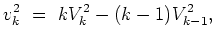where $v$ is the interval velocity, $V$ is the stacking velocity or RMS velocity, and $k$ is the sample number. Both velocities run down the traveltime depth axis. If we define $u_k=v^2_k$ and $d_k=kV_k^2$, we can set up the Dix inversion problem in an $L1$ sense as follows:

$$\vert\vert\boldsymbol{W_d}(\boldsymbol{C} \bold u-\bold d)\vert\vert _1 \approx 0,$$ (2)

where u is the unknown model we are inverting for, d is the known data from velocity scan, C is the causal integration operator, 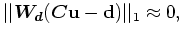$\bold W_d$ is a data residual weighting function, which is proportional to our confidence in the RMS velocity.

Fitting goal (2) itself cannot fully constrain the inversion problem, because the integration operator has a large null space at high frequencies. Therefore, Clapp et al. (1998) supplement this system with a regularization term to take the advantage of the prior geological information, of which smoothness and blockiness are two typical examples. For the case we are interested in, we use blockiness as regularization. In a mathematical form, it can be written as follows:

$$\vert\vert\epsilon \boldsymbol{D_{z}} \bold u \vert\vert _1\approx 0,$$ (3)

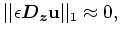where $\bold D_{z}$ is the vertical derivative of the velocity model and $\epsilon$ is the weight controlling the strength of the regularization.

Dix inversion constrained by L1-norm optimization