 |
 |
 |
 | Seismic tomography with co-located soft data |  |
![[pdf]](icons/pdf.png) |
Next: Application of the cross-gradient
Up: Maysami and Clapp: Constrained
Previous: The cross-gradient function: a
By definition, tomography is an inverse problem, in which a field
is reconstructed from its known linear path integrals, i.e.,
projections (Iyer and Hirahara, 1993; Clayton, 1984). Tomography can be represented by
a matrix operator
 , which integrates slowness along the raypath. The tomography problem can then be stated as
 |
(3) |
where
 and
and
 are traveltime and slowness vector, respectively (Clapp, 2001). The tomography operator is a function of the model parameters, since the raypaths depend on the velocity field. Consequently, the tomography problem is non-linear. A common technique to overcome this non-linearity is to iteratively linearize the operator around an a priori estimation of the slowness field
 (Clapp, 2001; Biondi, 1990; Etgen, 1990). The linearization of the tomography problem by using a Taylor expansion is given by
 |
(4) |
Here,
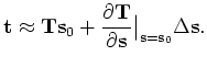 represents the update in the slowness field
with respect to the a priori slowness estimation,
. Equation
4 can be simplified as
represents the update in the slowness field
with respect to the a priori slowness estimation,
. Equation
4 can be simplified as
 |
(5) |
where
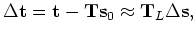 is a linear approximation of
. A second, but not lesser, difficulty arises because the locations of reflection points are unknown and are a function of the velocity field (Stork, 1992; van Trier, 1990).
is a linear approximation of
. A second, but not lesser, difficulty arises because the locations of reflection points are unknown and are a function of the velocity field (Stork, 1992; van Trier, 1990).
Clapp (2001) attempts to resolve some of the difficulties caused by the non-linearity of the seismic tomography problem by introducing a new tomography operator in the tau
domain and by using steering filters. In addition to geological models,
other types of geophysical data can also be extremely
important for yielding improved velocity estimates. In the following section, we show how the cross-gradient
function can be used to add constraints to the seismic tomography problem in order to decrease the uncertainties in the estimated velocity model.
|
|
|
|
| Seismic tomography with co-located soft data | |
|
Next: Application of the cross-gradient
Up: Maysami and Clapp: Constrained
Previous: The cross-gradient function: a
2009-06-03