Seismic tomography with co-located soft data

The cross-gradient function: a structural similarity measure

Integration of soft data into the seismic tomography problem can reduce model uncertainty and result in a better velocity estimation, especially in areas with complex structure. Different geophysical methods probs the same structures in the Earth's subsurface. Among the techniques for integrating different types of geological data, structural similarity-measurement tools may be a good choice for our tomography problem. The cross-gradient function is one tool that measures the structural similarity between any two fields. Following Gallardo and Meju (2004), we can define the cross-gradient function for the tomography problem as

$$\mathbf{g}=\nabla \mathbf{r} \times \nabla \mathbf{s},$$ (1)

where $\mathbf{r}$ and $\mathbf{s}$ can represent any two model parameters. In our case, they represent resistivity and slowness, respectively. Zero values of the cross-gradient function correspond to points where spatial changes in both geophysical properties, i.e., $\nabla \mathbf{r}$ and $\nabla \mathbf{s}$, align. However, the function is also zero where the magnitude of spatial variations of either field is negligible, e.g., where either property is smooth. Note that the cross-gradient function is a non-linear function of $\mathbf{r}$ and $\mathbf{s}$ if both are unknowns. In a 2-D problem, $\mathbf{g}$ simplifies to a scalar function at each point, given by

$$\mathbf{g}= \frac{\partial \mathbf{s}}{\partial x}  \frac{\parti... ...ac{\partial \mathbf{s}}{\partial z}  \frac{\partial \mathbf{r}}{\partial x} ,$$ (2)

where the model parameters are given in the $x-z$ plane. To compute the cross-gradient function, we can further simplify it by using first-order forward-differences approximations of the first derivative operators.

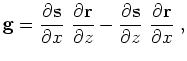
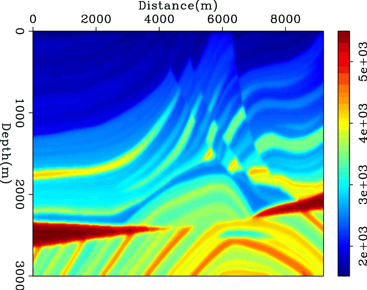
Figures 1(a) and 1(b) show the smooth Marmousi synthetic 2-D velocity model (Versteeg and Grau, 1991) and its cross-gradient with itself, respectively. The cross-gradient of a field with itself is called the auto-gradient hereafter. Note that the auto-gradient of a field should be zero everywhere; however, since the figures are prepared with a first-order linear approximation of the cross-gradient function, it is not zero, especially in areas with sharp edges.

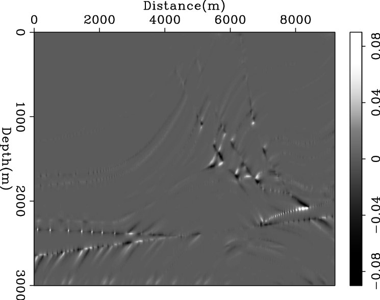
Although we expect different types of geophysical methods to result in similar structural maps, in practice each method maps the subsurface through different filters and frequency contents. Typical frequencies in magnetotelluric data are much lower than those of seismic data (Kaufman and Keller, 1981). This difference in the frequency content of two fields may affect how the cross-gradient represents the structural similarity of two fields. To investigate the effect of different spatial frequency content, we prepared Figure 1, in which the cross-gradient of the Marmousi velocity model and a smooth version of it is computed. In Figure 1(d), we have increased the smoothing factor. This increase is equivalent to a lower cut-off spatial frequency for a lowpass filter. Note that because of the relatively sharp edges in the original velocity model, the cross-gradients in Figures 1(c) and 1(d) seem to include some structure as well as higher amplitudes as compared with Figure 1(b). However, this synthetic example is an extreme case of complexity and sharp edges. As shown by the results for the Pillow velocity model in Figure 2, in simpler cases of subsurface structure, the cross-gradient with a smooth version of the velocity model leads to an acceptable similarity indicator. The amplitude may be improved by using a higher-order linear approximation of the cross-gradient computation. These figures in general may imply that the cross-gradient function can be used as a constraint for joint data inversion problems or to integrate a priori information from other fields into the seismic tomography problem.

marm-S0vel,marm-S0xg,marm-S1xg,marm-S2xg
Figure 1. Frequency sensitivity of the cross-gradient function: (a) The Marmousi velocity model; (b) its auto-gradient. Cross-gradient values of the Marmousi velocity model and its (c) smooth and (d) very smooth copies. [ER]

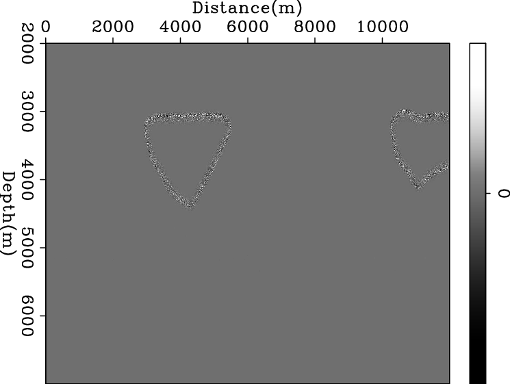
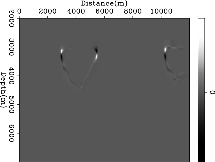
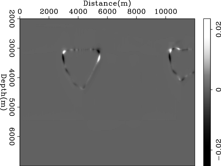
pilw-S0vel,pilw-S0xg,pilw-S1xg,pilw-S2xg
Figure 2. Frequency sensitivity of the cross-gradient function: (a) The Pillow velocity model; (b) its auto-gradient. Cross-gradient values of the Pillow velocity model and its (c) smooth and (d) very smooth copies. [ER]

Seismic tomography with co-located soft data