 |
 |
 |
 | Effective medium theory for elastic composites |  |
![[pdf]](icons/pdf.png) |
Next: RIGOROUS BOUNDS ON EFFECTIVE
Up: Berryman: Elastic composites theory
Previous: INTRODUCTION
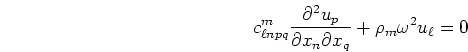
Mal and Knopoff (1967) derived an integral equation for the scattered displacement field
from a single elastic scatterer. Let  symbolize the volume of the region occupied by
a single inclusion
symbolize the volume of the region occupied by
a single inclusion  . Let the incident field be
 and let
 and
and
 be the total
field outside and inside the inclusion volume such that
be the total
field outside and inside the inclusion volume such that
 |
(1) |
The scattered fields are  and
and  . Both
 and
and
 satisfy the same equation:
 |
(2) |
outside the inclusion, while
 satisfies
 |
(3) |
inside the inclusion.
The indices 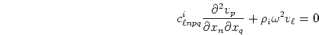 ,
, ,
, ,
, take the values
  for the three spatial dimensions,
and the Einstein summation convention applies in Equations (2) and (3),
and also throughout this paper.
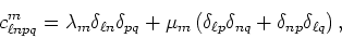
The elastic tensor for the matrix and inclusion are respectively:
for the three spatial dimensions,
and the Einstein summation convention applies in Equations (2) and (3),
and also throughout this paper.
The elastic tensor for the matrix and inclusion are respectively:
 |
(4) |
 |
(5) |
and  and
and
 are the respective densities.
Green's function for a point source in an infinite, isotropic, homogeneous elastic
medium of the matrix material is given by
![\begin{displaymath}
g_{pq}(\vec{x},\vec{\zeta}) = \frac{1}{4\pi\rho_m\omega^2}\l...
...(\frac{\exp{(ikr)}}{r} - \frac{\exp{(isr)}}{r}\right)\right],
\end{displaymath}](img27.png) |
(6) |
where
 ,
,
![$k = \omega[\rho_m/(\lambda_m+2\mu_m)]^{1/2}$](img29.png) ,
and
,
and
![$s = \omega[\rho_m/\mu_m]^{1/2}$](img30.png) -- with
-- with 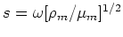 and
and  being, respectively, the magnitudes of the wavevectors for
compressional and shear waves in the matrix. Given the form of
being, respectively, the magnitudes of the wavevectors for
compressional and shear waves in the matrix. Given the form of  , Mal and Knopoff (1967)
then derive an integral equation for
. Since the derivation follows
standard lines of argument, I will not repeat it here. The result is
, Mal and Knopoff (1967)
then derive an integral equation for
. Since the derivation follows
standard lines of argument, I will not repeat it here. The result is
![\begin{displaymath}
u_\ell(\vec{x}) = u^0_\ell(\vec{x})
+\int_{\Omega_i}d\vec{\z...
...tial}{\partial\zeta_j}\right]g_{\ell n}(\vec{x},\vec{\zeta}).
\end{displaymath}](img34.png) |
(7) |
Equation (7) is an exact integral equation for the displacement field in the
region exterior to the scatterer in terms of the displacement and strain fields inside
the inclusion volume .
To evaluate the integral (7), estimates of the interior displacement and strain fields
are required. Considering the first Born approximation from quantum scattering theory suggests the
estimates for wave speed and strain at
 :
:
 |
(8) |
and
 |
(9) |
By Equations (8) and (9), I mean to approximate  and
and  by the
values
by the
values  and
and  would have achieved at position
  if the matrix
contained no scatterers. For scatterers with small volumes, it follows from (7) that
if the matrix
contained no scatterers. For scatterers with small volumes, it follows from (7) that
 and its derivatives are small quantities for
  outside of .
Since the displacement is continuous across the boundary, it follows that Equation (8) will
be a good approximation to
outside of .
Since the displacement is continuous across the boundary, it follows that Equation (8) will
be a good approximation to
 . However, this argument fails for Equation (9),
because the strains are not continuous across the boundary. Equation (9) should therefore be
replaced by the formula:
. However, this argument fails for Equation (9),
because the strains are not continuous across the boundary. Equation (9) should therefore be
replaced by the formula:
 |
(10) |
where  is Wu's tensor [Wu (1966)], relating
  for an arbitrary ellipsoidal inclusion
to the uniform strain at infinity
for an arbitrary ellipsoidal inclusion
to the uniform strain at infinity
 .
Now, if the wavelength of the incident waves is large compared to the size of the ellipsoid
(i.e.,
.
Now, if the wavelength of the incident waves is large compared to the size of the ellipsoid
(i.e.,
 , where
  is the wavelength), then the fields both near
the ellipsoid and inside scatterer volume will be essentially static and uniform
[Eshelby (1957)].
Thus, to the lowest order of approximation, it is valid to make the
substitutions (8) and (10). When the ellipsoid is centered at
is the wavelength), then the fields both near
the ellipsoid and inside scatterer volume will be essentially static and uniform
[Eshelby (1957)].
Thus, to the lowest order of approximation, it is valid to make the
substitutions (8) and (10). When the ellipsoid is centered at  ,
it follows easily that
,
it follows easily that
![\begin{displaymath}
u_{\ell}^s(\vec{x}) = \Omega_i\left[\Delta\rho_i\omega^2u_n^...
...t)
\epsilon_{rs}^0g_{\ell n,j}(\vec{x},\vec{\zeta}_i)\right],
\end{displaymath}](img53.png) |
(11) |
where the symmetry properties of have been used in simplifying the expression. A comma preceding
a subscript indicates a derivative with respect to the as-labelled component.
Equation (11) gives the first order estimate of the scattered wave from an ellipsoidal
inclusion whose principal axes are aligned with the coordinate axes. When the ellipsoid is oriented
arbitrarily with respect to the coordinate axes, Equation (11) must be changed
by replacing  everywhere with
 |
(12) |
where
 are the appropriate direction cosines. For homogeneous,
isotropic composites with randomly oriented ellipsoidal inclusions,
the general form of the average tensor as given by Wu (1966) is
are the appropriate direction cosines. For homogeneous,
isotropic composites with randomly oriented ellipsoidal inclusions,
the general form of the average tensor as given by Wu (1966) is
 |
(13) |
where
 |
(14) |
Finally, suppose  inclusions are contained in a small volume of
radius
inclusions are contained in a small volume of
radius  centered at
  . Assume that the effects of multiple
scattering may be neglected at sufficiently low frequencies (i.e., long wavelengths appropriate for seismology)
to the lowest order. Then, to the same degree of approximation used
in Equation (11) (i.e.,
), the scattered wave
has the form:
. Assume that the effects of multiple
scattering may be neglected at sufficiently low frequencies (i.e., long wavelengths appropriate for seismology)
to the lowest order. Then, to the same degree of approximation used
in Equation (11) (i.e.,
), the scattered wave
has the form:
![\begin{displaymath}
\left<u_\ell^s(\vec{x})\right>^m \simeq \sum_{i=1}^N \Omega_...
...ht)\epsilon_{rs}^0g_{\ell n,j}(\vec{x},\vec{\zeta}_0)\right],
\end{displaymath}](img62.png) |
(15) |
where the superscripts  and again refer to matrix and inclusion properties, respectively.
Note especially that distinct superscripts must be used in Equation (15)
to specify both the inclusion material itself, and also the shape of each distinct type
of inclusion.
and again refer to matrix and inclusion properties, respectively.
Note especially that distinct superscripts must be used in Equation (15)
to specify both the inclusion material itself, and also the shape of each distinct type
of inclusion.
To apply this thought experiment to the analytical problem of estimating
elastic constants, consider replacing the true composite sphere with a sphere
composed of matrix material identical to the imbedding material and of
ellipsoidal inclusions of the same materials as those in the true composite, and also
in the same proportions. Then, if multiple scattering effects may be (and are) neglected, the
theoretical expression which determines the elastic constants is
 |
(16) |
where the left hand side is given by Equation (15) with matrix-type  .
Equation (16) states simply that the net (overall) scattering -- due to many scatterers - in the self-consistently
determined medium vanishes to lowest order.
.
Equation (16) states simply that the net (overall) scattering -- due to many scatterers - in the self-consistently
determined medium vanishes to lowest order.
If the volume fraction of the -th component is defined by
 , then
Equation (16) implies the following formulas:
, then
Equation (16) implies the following formulas:
 |
(17) |
 |
(18) |
and
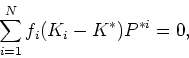 |
(19) |
Equation (17) states that the effective density 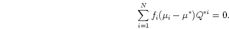 is just the
volume average density (which is what one might reasonably expect, but nevertheless is not always
true for effective medium theories).
Equations (18) and (19) provide implicit
formulas for
is just the
volume average density (which is what one might reasonably expect, but nevertheless is not always
true for effective medium theories).
Equations (18) and (19) provide implicit
formulas for  and
and  . Such implicit formulas are typically solved
numerically by iteration [Berryman (1980b)]. This step is usually necessary because
the factors
. Such implicit formulas are typically solved
numerically by iteration [Berryman (1980b)]. This step is usually necessary because
the factors  and
and  are themselves both typically functions
of both the unknown quantities and . Experience has shown that
such iterative methods often converge in a stable fashion, and usually after a small number of iterations
(typically 10 or less).
are themselves both typically functions
of both the unknown quantities and . Experience has shown that
such iterative methods often converge in a stable fashion, and usually after a small number of iterations
(typically 10 or less).
The derivation given and final results attained here are very similar to methods
discussed by Elliott et al. (1974) and
Gubernatis and Krumhansl (1975).
I will therefore refer to the resulting effective medium method as the ``coherent potential
approximation'' (or CPA), as is typically done in the physics literature,
since the early work of Soven (1967). Equations (18) and (19)
were also obtained independently by Korringa et al. (1979), while using an entirely different method. In the following sections, I will compare
the results obtained from this effective medium theory to the known
rigorous bounds on elastic constants and also to the results
of other effective medium theories.
|
|
|
|
| Effective medium theory for elastic composites | |
|
Next: RIGOROUS BOUNDS ON EFFECTIVE
Up: Berryman: Elastic composites theory
Previous: INTRODUCTION
2009-05-05