Effective medium theory for elastic composites

RIGOROUS BOUNDS ON EFFECTIVE MODULI

In their review article, Watt et al. (1976) discuss various rigorous bounds on the effective moduli of composites. For example, the well-known Voigt (arthimetic) and Reuss (harmonic) averages are, respectively, rigorous [Hill (1952)] upper and lower bounds for both $K^*$ and $\mu^*$. Generally tighter bounds have also been given by Hashin and Shtrikman (1963,1961,1962).

Still tighter bounds have been obtained in principle by Beran and Molyneux (1966) for the bulk modulus and by McCoy (1970) for the shear modulus. However, the resulting formulas depend on three-point spatial correlation functions for the composite and are therefore considerably more difficult to evaluate than the expressions for the Hashin-Shtrikman [Hashin and Shtrikman (1963,1961,1962)] bounds, which depend only on the material constants and volume fractions. Miller (1969a,b) evaluated the bounds of Beran and Molyneux (1966) by treating an isotropic homogeneous distribution of statistically independent cells. Silnutzer (1972) used the same approach to simplify the bounds of McCoy (1970) for cell materials. Furthermore, Milton (1981) has shown that the bounds of Beran and Molyneux (1966) and McCoy (1970) can be simplified somewhat even if the composite is not a cell material. Nevertheless, the bounds which are most easily evaluated are still the Hashin-Shtrikman [Hashin and Shtrikman (1963,1961,1962)] (HS) bounds, the Beran-Molyneux-Miller (BMM) bounds, and the McCoy-Silnutzer (MS) bounds. I will compare these bounds to the estimates obtained from the coherent potential approximation (CPA), the specific effective medium theory being stressed here.

To aid in the following comparisons, it is convenient to introduce two functions:

$$\Lambda(x) = \left(\sum_{i=1}^N \frac{f_i}{K_i + 4x/3}\right)^{-1} - \frac{4}{3}x,$$ (20)

$$\Gamma(y) = \left(\sum_{i=1}^N \frac{f_i}{\mu_i + y}\right)^{-1} - y,$$ (21)

together with a third function that is needed in conjunction with $\Gamma$:

$$F(x,z) = \frac{x}{6}\left(\frac{9z+8x}{z+2x}\right).$$ (22)

It has been shown previously [Berryman (1980b,1995)] that $\Lambda(x)$ and $\Gamma(y)$ are monotonically increasing functions of their real arguments. Similarly, I find that

$$\frac{\partial F}{\partial z} = \frac{5x^2}{3(z+2x)^2} \ge 0$$ (23)

and

$$\frac{\partial F}{\partial x} = \frac{9z^2 + 16xz + 16x^2}{6... ...2} \ge 0 \quad\hbox{if}\quad x \ge 0, \quad \& \quad z \ge 0.$$ (24)

So, when both arguments of $F(x,z)$ are non-negative (which will soon be shown to be the case in these applications), it follows that $F$ is a monotonically increasing function of both arguments.

Now, if I define the minimum and maximum moduli among all the constitutents by

$$\begin{array}{cc} K_+ = \max{(K_1,\ldots,K_N)}, & \quad K_- ... ...u_N)}, & \quad \mu_- = \min{(\mu_1,\ldots,\mu_N)}, \end{array}$$ (25)

then the Hashin-Shtrikman bounds are also given in general by

$$K_{HS}^\pm = \Lambda\left(\mu_\pm\right)$$ (26)

and

$$\mu_{HS}^\pm = \Gamma\left[F\left(\mu_\pm,K_\pm\right)\right].$$ (27)

[Note that the only combinations considered on the right-hand side of (27) are those having both pluses or both minuses - no mixing of the subscripts.]

The Beran-Molyneux-Miller bounds and the McCoy-Silnutzer bounds are known for two-phase composites (i.e., $N = 2$). These bounds can be written in succinct form using the notation of Milton (1981). By defining two geometric parameters $\zeta_1 = 1 - \zeta_2$ and $\eta_1 = 1 - \eta_2$, and two related averages [analogous to the volume fraction weighted average $\left<M\right> = f_1M_1 + f_2M_2$] of any modulus $M$ by $\left<M\right>_\zeta = \zeta_1M_1 + \zeta_2M_2$, and $\left<M\right>_\eta = \eta_1M_1 + \eta_2M_2$, then the bounds can be written very concisely as:

$$K_{BMM}^+ = \Lambda\left(\left<\mu\right>_\zeta\right),$$ (28)

$$K_{BMM}^- = \Lambda\left(\left<1/\mu\right>^{-1}_\zeta\right),$$ (29)

$$\mu_{MS}^+ = \Gamma(\Theta/6),$$ (30)

and

$$\mu_{MS}^- = \Gamma(\Xi^{-1}/6),$$ (31)

where

$$\Theta = \left[10\left<\mu\right>^2\left<K\right>_\zeta + 5\... ...u\right>^2 \left<\mu\right>_\eta\right]/\left<K+2\mu\right>^2$$ (32)

and

$$\Xi = \left[10\left<K\right>^2\left<\frac{1}{K}\right>_\zeta... ...left<\frac{1}{\mu}\right>_\eta\right]/\left<9K+8\mu\right>^2.$$ (33)

For symmetric cell materials, it is known that $\zeta_1 = \eta_1 = f_1$ for spherical cells, $\zeta_1 = \eta_1 = f_2$ for disks, while $\zeta_1 = (3f_1 + f_2)/4$, and $\eta_1 = (5f_1+f_2)/6$ for needles.

It is particularly simple to compare these bounds with the results of effective medium theory when the inclusions are assumed to be spherical in shape. Then, the estimates of the moduli are given by the self-consistent formulas (which are mutually interdependent):

$$K^* = \Lambda(\mu^*)$$ (34)

and

$$\mu^* = \Gamma\left[F\left(\mu^*,K^*\right)\right].$$ (35)

Furthermore, the bounds (28)-(30) simplify in this case and are given by

$$K_{BMM}^+ = \Lambda\left(\left<\mu\right>\right),$$ (36)

$$K_{BMM}^+ = \Lambda\left(\left<1/\mu\right>^{-1}\right),$$ (37)

and

$$\mu_{MS}^+ = \Gamma\left[F\left(<\mu>,<K>\right)\right].$$ (38)

From the monotonicity properties of the functions (20)-(22), from elementary arguments relating the estimates to the Voigt and Reuss averages, and also from the fact that all the arguments of these functions depend on quantities composed of elastic constants averaged using positive measures such as volume fractions and the related quantities for various cell-material shapes, I find for the bulk modulus that

$$\Lambda(\mu_-) \le \Lambda\left(\left<1/\mu\right>^{-1}\righ... ... \le \Lambda\left(\left<\mu\right>\right) \le \Lambda(\mu_+),$$ (39)

or equivalently that

$$K_{HS}^- \le K_{BMM}^- \le K^* \le K_{BMM}^+ \le K_{HS}^+.$$ (40)

Similarly, by making use of $\Gamma(y)$ from (21), it follows for the shear modulus that

$$\mu_{HS}^- \le \mu^* \le \mu_{MS}^+ \le \mu_{HS}^+.$$ (41)

The detailed argument leading to Equation (39) is a little involved: First, I must show that $K^*$, $\mu^*$ are bounded by the Hashin-Shtrikman bounds [Berryman (1980a)]. Then, since the Hashin-Shtrikman bounds are themselves bounded by the Voigt and Reuss bounds, Equation (39) follows from

$$\Lambda(\left<1/\mu\right>^{-1}) \le \Lambda(\mu^-_{HS}) \le... ...\mu^*) \le \Lambda(\mu^+_{HS}) \le \Lambda(\left<\mu\right>).$$ (42)

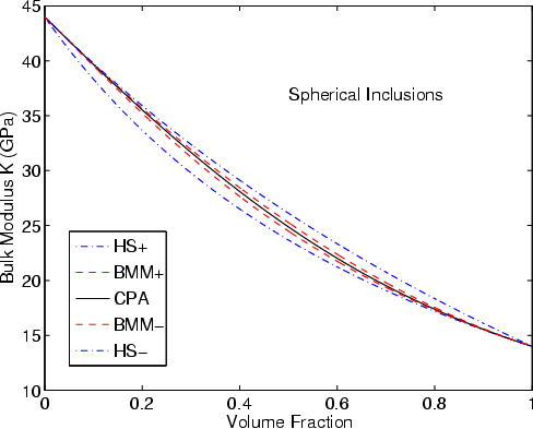
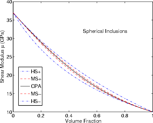
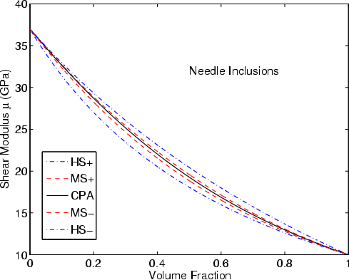
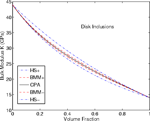
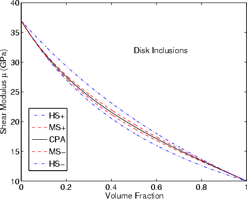
The arguments just given are valid only for the case of spherical inclusions. The author knows of no general argument relating the effective medium results to the rigorous bounds for arbitrary inclusion shapes. However, as will be observed in the following Figures, numerical examples illustrate the effective medium estimates always lying between the bounds.

K-SPH,G-SPH
Figure 1. Estimates of the effective bulk (a) and shear (b) moduli of elastic composites with constituents $K_1 = 44.0$ GPa, $\mu _1 = 37.0$ GPa, $K_2 = 14.0$ GPa, and $\mu _2 = 10.0$ GPa as the volume fraction of type-2 increases. The curves are respectively the CPA (or coherent potential approximation: a self-consistent estimator) -- which is the black solid line, the Beran-Molyneux-Miller bounds for the bulk modulus and the McCoy-Silnutzer bounds for the shear modulus -- which are the red dashed lines, and the Hashin-Shtrikman bounds -- which are the blue dot-dashed lines. Inclusions are treated as having spherical shape. NR

K-NDL,G-NDL
Figure 2. Estimates of the effective bulk (a) and shear (b) moduli of elastic composites with constituents $K_1 = 44.0$ GPa, $\mu _1 = 37.0$ GPa, $K_2 = 14.0$ GPa, and $\mu _2 = 10.0$ GPa as the volume fraction of type-2 increases. The curves are respectively the CPA (or coherent potential approximation: a self-consistent estimator) -- which is the black solid line, the Beran-Molyneux-Miller bounds for the bulk modulus and the McCoy-Silnutzer bounds for the shear modulus -- which are the red dashed lines, and the Hashin-Shtrikman bounds -- which are the blue dot-dashed lines. Inclusions are treated here as having needle-like shape. NR

K-DSK,G-DSK
Figure 3. Estimates of the effective bulk (a) and shear (b) moduli of elastic composites with constituents $K_1 = 44.0$ GPa, $\mu _1 = 37.0$ GPa, $K_2 = 14.0$ GPa, and $\mu _2 = 10.0$ GPa as the volume fraction of type-2 increases. The curves are respectively the CPA (or coherent potential approximation: a self-consistent estimator) -- which is the black solid line, the Beran-Molyneux-Miller bounds for the bulk modulus and the McCoy-Silnutzer bounds for the shear modulus -- which are the red dashed lines, and the Hashin-Shtrikman bounds -- which are the blue dot-dashed lines. Inclusions are treated here as having disk-like shape. NR

Typical results are presented in Figures 1-3. The values of the constituents' moduli were chosen to be: $K_1 = 44.0$ GPa, $\mu _1 = 37.0$ GPa, $K_2 = 14.0$ GPa, and $\mu _2 = 10.0$ GPa. The values of $K_2$ and $\mu_2$ were chosen as a compromise between two extremes: (a) If $K_2$ and $\mu_2$ are too close to $K_1$ and $\mu_1$, then the bounds are too close together to be distinguishable on the plots. (b) If $K_2$ and $\mu_2$ are both chosen to be zero, the iteration to the effective medium theory results does not converge for the case of disk-like inclusions [Berryman (1980b)], although all the other cases converge without difficulties. I find in all cases considered that the effective medium theory results lie between the rigorous bounds, as stated above.

Effective medium theory for elastic composites