 |
 |
 |
 | Delayed-shot migration in TEC coordinates |  |
![[pdf]](icons/pdf.png) |
Next: Impulse response tests
Up: Shragge: 3D imaging in
Previous: TEC extrapolation wavenumber
One obvious concern is whether the dispersion relationship in equation 16 can be implemented accurately and efficiently in a wavefield extrapolation scheme. I address this question by comparing the elliptical-cylindrical dispersion relationship to that for elliptically anisotropic media in Cartesian coordinates. By defining an effective slowness  and rewriting equation 16 as
 |
(19) |
the TEC coordinate dispersion relationship resembles that of elliptically anisotropic media (Tsvankin, 1996). More specifically, extrapolation in TEC coordinates is related to a special case where the Thomsen parameters (Thomsen, 1986) obey
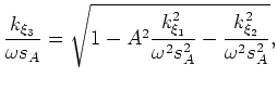 :
:
 |
(20) |
From equation 20 we see that equation 16 is no more complex than the dispersion relationship for propagating waves in elliptically anisotropic media, which is now routinely handled with finite-difference approaches (Zhang et al., 2001; Baumstein and Anderson, 2003; Shan and Biondi, 2005).
A general approach to 3D implicit finite-difference propagation is to approximate the square-root by a series of rational functions (Ma, 1982)
 |
(21) |
where
 and
and
 , for
, for 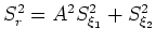 , and
, and  is the order of the coefficient expansion.
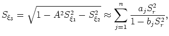
An optimal set of coefficients can be found by solving an optimization problem (Shan and Biondi, 2005),
![$\displaystyle E(a_j,b_j) = {\rm min} \int_{0}^{{\rm sin} \phi} \left[ \sqrt{1-S_r^2} - \sum_{j=1}^{n} \frac{a_j S_r^2}{1 - b_j S_r^2} \right]^2 {\rm d}S_r,$](img99.png) |
(22) |
where 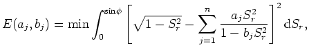 is the maximum optimization angle. I generated the following results using a 4th-order approximation and coefficients found in Table 1 (Lee and Suh, 1985).
Table 1:
Coefficients used in 3D implicit finite-difference wavefield extrapolation.
Coeff. order  |
Coeff.  |
Coeff.  |
| 1 |
0.040315157 |
0.873981642 |
| 2 |
0.457289566 |
0.222691983 |
|
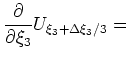
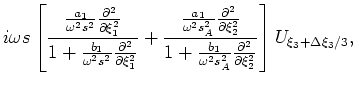
Specifying a finite-difference extrapolator operator using the 4th-order approximation is equivalent to solving a cascade of partial differential equations (Shan and Biondi, 2005)
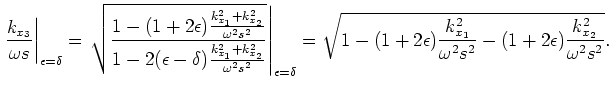
I solve these equations implicitly at each extrapolation step by a finite-difference splitting approach that alternatively advances the wavefield in the  and
and  directions. Splitting methods allow the direct application of the
  scaling factor in equation 21 by introducing the original slowness model,
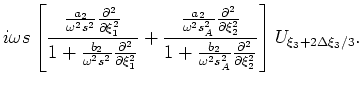 , for the direction split.
One drawback to finite-difference splitting methods is that they commonly generate numerical anisotropy. To minimize these effects, I apply a Fourier-domain phase-correction filter ![$ L[\cdot]$](img110.png) (Li, 1991)
(Li, 1991)
![$\displaystyle L[U] = U{\rm e}^{ i \Delta \xi_3 k_L},$](img111.png) |
(24) |
where
![$\displaystyle k_L = \sqrt{ 1-\frac{k_{\xi_1}^2}{(\omega s_1^r)^2} -\frac{k_{\xi...
...}{\omega s_2^r})^2}{1-b_j ( \frac{k_{\xi_2}}{\omega s_2^r})^2} \right) \right],$](img112.png) |
(25) |
and 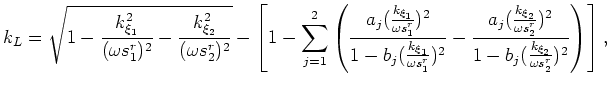 and
and  are reference slownesses chosen to be the
mean value of
are reference slownesses chosen to be the
mean value of  and
and 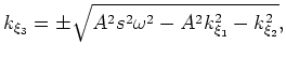 defined above, respectively. Note that while this phase-shift correction is explictly correct for v(
 ) media, the Li filter in v(
 ) media is only approximate and will introduce error.
Subsections
|
|
|
|
| Delayed-shot migration in TEC coordinates | |
|
Next: Impulse response tests
Up: Shragge: 3D imaging in
Previous: TEC extrapolation wavenumber
2009-05-05
![$\displaystyle i \omega s
\left[
\frac{ \frac{a_1}{\omega^2s^2} \frac{\partial^2...
...^2s_A^2} \frac{\partial^2}{\partial \xi_2^2}
}
\right] U_{\xi_3+\Delta\xi_3/3},$](img106.png)
![$\displaystyle i \omega s
\left[
\frac{ \frac{a_2 }{\omega^2s^2} \frac{\partial^...
...^2s_A^2}\frac{\partial^2}{\partial \xi_2^2} }
\right] U_{\xi_3+2\Delta\xi_3/3}.$](img108.png)