Delayed-shot migration in TEC coordinates

TEC extrapolation wavenumber

A metric tensor $g_{jk}$ can be specified from the mapping relationship given in equations 13:

$$\left[g_{jk}\right] = \left[\begin{array}{ccc} 1 & 0 & 0 0 & A^2 & 0 0 & 0 & A^2 \end{array}\right],$$ (14)

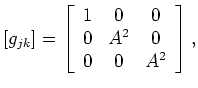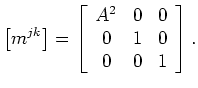
where $A=a \sqrt{ {\rm sinh}^2 \xi_3 + {\rm sin}^2 \xi_2 }$. The determinant of the metric tensor is: $\vert\boldsymbol{g}\vert = A^4$. The corresponding inverse weighted metric tensor, $m^{jk}$ as developed in Shragge (2008), is given by:

$$\left[m^{jk}\right] = \left[\begin{array}{ccc} A^2 & 0 & 0 0 & 1 & 0 0 & 0 & 1 \end{array}\right].$$ (15)

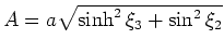
Note that even though the metric of the TEC coordinate system varies spatially, the local curvature parameters ( $n^j=\frac{\partial m^{jk}}{\partial\xi_k}$) remain constant: $n^1=n^2=n^3=0$. The corresponding extrapolation wavenumber, $k_{\xi_3}$, can be generated by inputting tensor $m^{jk}$ and fields $n^j$ into the general wavenumber expression for 3D non-orthogonal coordinate systems

$$k_{\xi_3} = \pm \sqrt{ A^2 s^2 \omega ^2 - A^2 k_{\xi_1}^2 - k_{\xi_2}^2 },$$ (16)

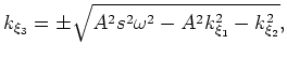where $s$ is the slowness (reciprocal of velocity), $k_{\xi_3}$ is the extrapolation wavenumber, and $k_{\xi_1}$ and $k_{\xi_2}$ are the inline and crossline wavenumbers, respectively.

The wavenumber specified in equation 16 is central to the inline delayed-shot migration algorithm. The first step is to extrapolate the source and receiver wavefields

$$E_{\xi_3}[S_{jl} (\xi_3,\xi_1,\xi_2\vert\omega ) ] = S_{jl} (\xi_3+\Delta \xi_3, \xi_1,\xi_2\vert\omega ),$$ (17)

$$E^*_{\xi_3} [R_{kl} (\xi_3,\xi_1,\xi_2\vert\omega ) ] = R_{kl} (\xi_3+\Delta \xi_3,\xi_1,\xi_2\vert\omega ),$$ (18)

where $E_{\xi_3}[\cdot]$ and $E^*_{\xi_3}[\cdot]$ are the extrapolation operator and its conjugate, respectively. The results herein were computed using the $\omega-\xi$ finite-difference extrapolators discussed below. The second step involves summing the individual inline delayed-shot images contributions, $I^{DS}_{jk} (\boldsymbol{\xi})$, into the total image volume, $I(\boldsymbol{\xi})$ according to equation 12.

Delayed-shot migration in TEC coordinates