Target-oriented joint inversion of incomplete time-lapse seismic data sets

Sparse data problem

This example demonstrates a particular sparse time-lapse seismic monitoring problem (Arogunmati and Harris, 2007), where sparse randomly-sampled monitor data sets are acquired at a fraction of the cost of the full survey. Here, we consider a full baseline data set and three randomly sampled monitor surveys each constituting only 25 percent--at 50 per cent source and receiver sampling--of the full data set (Figure 3).

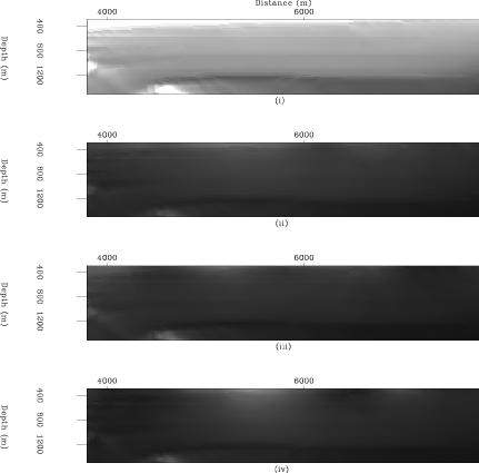
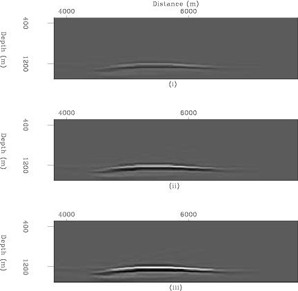
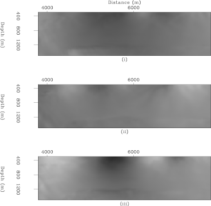
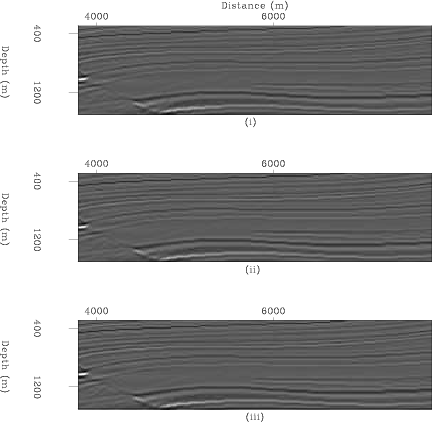
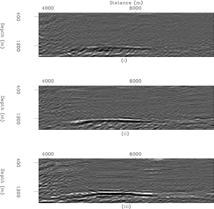
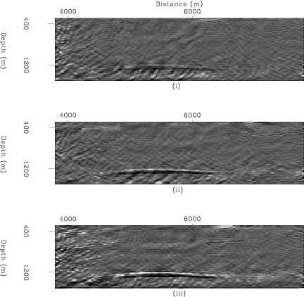
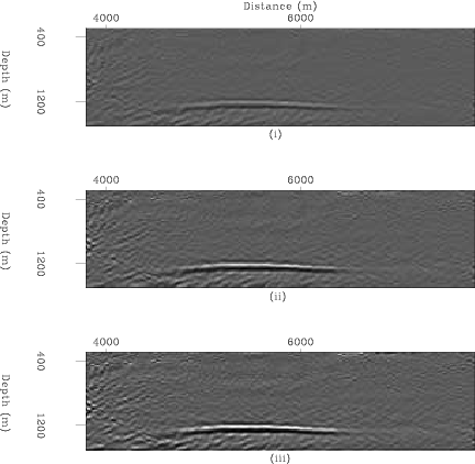
Migrated images of the target area are shown in Figure 6(a), and the corresponding Hessian diagonals in Figure 6(b). Figure 6(c) shows the cumulative time-lapse images of the target area obtained from the full data sets, and Figure 6(d) the illumination ratio between monitor and baseline data sets. The migrated, normalized, separately and jointly inverted time-lapse images are shown in Figure 7. Note that the migrated and normalized time-lapse images [Figures 7(a) and 7(b)] show no resemblance to the full data results [Figure 6(c)]. Also, note that time-lapse images obtained from joint inversion [Figure 7(d)] contain fewer artifacts than those from separate invertion [Figure 7(c)].

migs-1w-r,illums-hole-1w-r,migs-4d-1w2,illums-hole-r-1w-r
Figure 6. (a) Migrated (i) baseline and (ii)-(iv) monitor images. (b) Hessian diagonal corresponding to images in (a). (c) Cumulative time-lapse images from full baseline and monitor shot-receiver coverage [Figure 2(a)]. (d) Illumination-ratio for each monitor survey [Figures b(ii)-(iv)] relative to the baseline [Figure b(i)].[CR]

migs-4d-1w-r,invd-4d-1w-r,invs-4d-1w-r,inv2-4d-1w-r
Figure 7. Cumulative time-lapse images at four production stages (with increasing production from top to bottom) obtained from (a) migration, (b) Hessian-diagonal illumination correction, (c) separate inversion, and (d) RJMI. Compare these results to those from the full data sets [Figure 6(c)].[CR]

Target-oriented joint inversion of incomplete time-lapse seismic data sets