|
|
|
|
Target-oriented joint inversion of incomplete time-lapse seismic data sets |
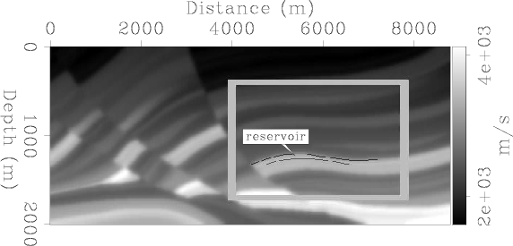
We consider two incomplete synthetic time-lapse seismic examples aimed at imaging seismic amplitude changes using incomplete time-lapse seismic data sets. Both examples are based on a modified section of the Marmousi model (Figure 1) with the target reservoir located at a shallower depth than the original Marmousi reservoir. In both examples, we neglect geomechanical changes above the reservoir.
In both cases, the baseline data set consists of ![]() surface shots spaced at
surface shots spaced at ![]() m and
m and ![]() receivers spaced at
receivers spaced at ![]() m.
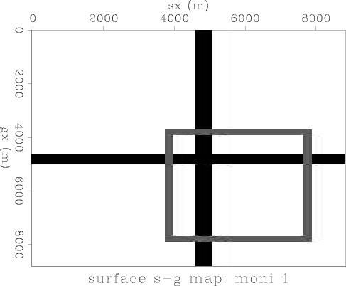
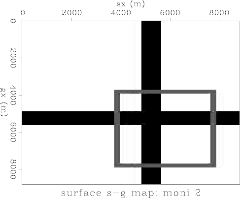
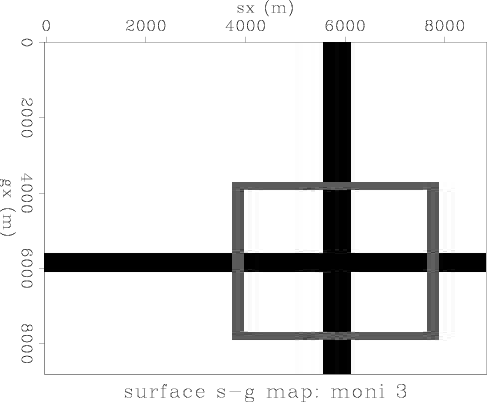
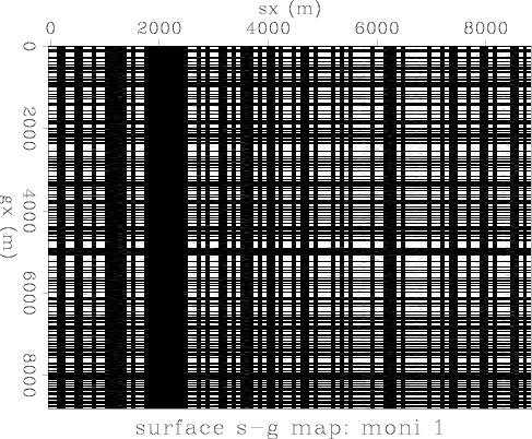
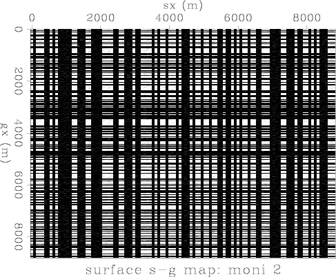
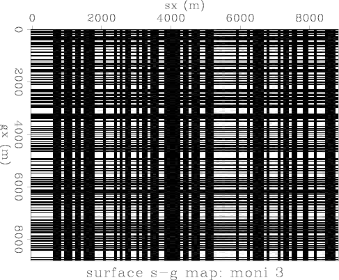
In the first example, the monitor data sets were modeled with gaps in data created by obstructions along the survey line (Figure 2).
The monitor data sets in the second example consist of randomly sampled shot and receiver axis (Figure 3).
We avoid a multiple attenuation requirement by using a Born single-scattering modeling algorithm.
We migrated the data sets with the oneway wave-equation, using 184 frequencies and computed the target-oriented Hessian with 72 frequencies.
m.
In the first example, the monitor data sets were modeled with gaps in data created by obstructions along the survey line (Figure 2).
The monitor data sets in the second example consist of randomly sampled shot and receiver axis (Figure 3).
We avoid a multiple attenuation requirement by using a Born single-scattering modeling algorithm.
We migrated the data sets with the oneway wave-equation, using 184 frequencies and computed the target-oriented Hessian with 72 frequencies.
We compare the results from migration, normalization with the Hessian diagonal, separate, and joint inversion for the target area in Figure 1. Normalization with the Hessian diagonal is one implementation of the so-called true-amplitude migration (Gray, 1997). In both examples, the same spatial regularization parameters were used for the separately and jointly inverted results. Where applicable, the regularization operators are Laplacian in x-direction and first-order gradient in time.
|
|---|
|
vel-pick3
Figure 1. Modified section of the Marmousi velocity model showing the reservoir location. The gray box shows the target area.[ER] |
|
|

|
|---|
|
map0-h,map1-h,map2-h,map3-h
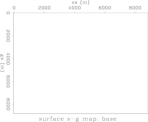
Figure 2. Surface shot-geophone coverage maps for the (a) baseline and (b)-(d) monitor surveys. White indicates locations with shot-receiver coverage whereas black gaps indicate the undershoot positions. The gray box indicates the surface location of the target area in both this Figure and also in Figure 3.[ER] |
|
|
|
|---|
|
map0-r,map1-r,map2-r,map3-r
Figure 3. Surface shot-geophone coverage maps for the (a) baseline and (b)-(d) monitor surveys. White indicates locations with shot-receiver coverage whereas black indicates no coverage.[ER] |
|
|
|
|
|
|
Target-oriented joint inversion of incomplete time-lapse seismic data sets |