|
|
|
|
Target-oriented joint inversion of incomplete time-lapse seismic data sets |
Given two data sets (baseline and monitor), acquired over an evolving earth model at times ![]() and
and ![]() respectively, we can write
respectively, we can write
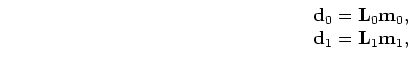 and
and
Applying the adjoint operators
![]() and
and
![]() to
to
![]() and
and
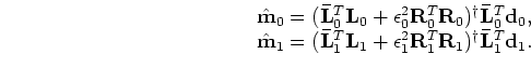
![]() respectively, we obtain the migrated baseline
respectively, we obtain the migrated baseline
![]() and monitor
and monitor
![]() images:
images:
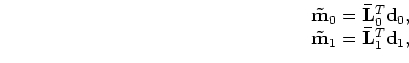 denotes conjugate transpose of
Because incomplete seismic data sets leads to high non-repeatability,
![]() and
and
![]() must be cross-equalized before
must be cross-equalized before
![]() is computed.
The high level of non-repeatability makes it difficult to adapt existing cross-equalization methods (Rickett and Lumley, 2001; Calvert, 2005; Hall, 2006) to randomly sampled time-lapse seismic data sets.
The RJMI method takes the data acquisition geometry and sampling into account and hence can correct for the non-repeatability of the data sets.
is computed.
The high level of non-repeatability makes it difficult to adapt existing cross-equalization methods (Rickett and Lumley, 2001; Calvert, 2005; Hall, 2006) to randomly sampled time-lapse seismic data sets.
The RJMI method takes the data acquisition geometry and sampling into account and hence can correct for the non-repeatability of the data sets.
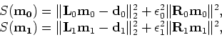
We define two quadratic cost functions for the modeling experiments (equation 2):
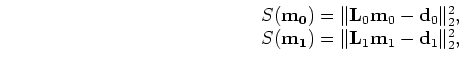 and
and
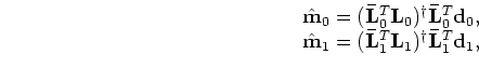 denotes approximate inverse.
Because seismic inversion is ill-posed, model regularization is often required to ensure stability and convergence to a geologically consistent solution.
For many seismic monitoring objectives, the known geology and reservoir architecture provide useful regularization information.
Including baseline and monitor regularization operators (
![]() and
and
![]() respectively) in the cost functions gives
respectively) in the cost functions gives
 is a regularization parameter that determines the strength of the regularization relative to the data fitting goal.
Although there is a wide range of suggested methods for selecting
, in most practical applications, the final choice of the parameter is subjective.
Unless otherwise stated, we use a fixed, heuristically determined, data-dependent regularization parameter given by
or
is a regularization parameter that determines the strength of the regularization relative to the data fitting goal.
Although there is a wide range of suggested methods for selecting
, in most practical applications, the final choice of the parameter is subjective.
Unless otherwise stated, we use a fixed, heuristically determined, data-dependent regularization parameter given by
or
Substituting equation 3 into equation 8, and re-arranging the terms, we get
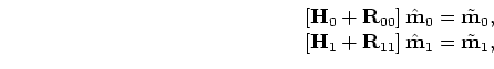 is the Hessian, and
An inverted time-lapse image,
![]() , can be obtained as the difference between the two images,
, can be obtained as the difference between the two images,
![]() and
and
![]() :
:
|
|
|
|
Target-oriented joint inversion of incomplete time-lapse seismic data sets |
![\begin{displaymath}\begin{array}{cc} \left [ {\bf H}_{0}+{\bf R}_{00} \right ] \...
...11} \right ] \hat{{\bf m}}_{1}= \tilde {\bf m}_{1}, \end{array}\end{displaymath}](img37.png)