Target-oriented joint inversion of incomplete time-lapse seismic data sets

Joint inversion of multiple images

In order to solve a single joint inversion problem in which the baseline and monitor images are simultaneously estimated, we combine the two expressions in equation 2 to get

$$\left [ \begin{array}{cc} {\bf d}_{0} {\bf d}_{1} \end{array} ... ...ht ] \left [ \begin{array}{cc} {\bf m}_{0} {\bf m}_{1} \end{array} \right ],$$ (A-12)

which can be solved by minimizing the cost function

$$\begin{array}{ccc} S({\bf m_{0}}, {\bf m_{1}})= \left \vert\l... ...rray} \right ] \right \vert \right \vert ^2_{2}, \end{array}$$ (A-13)

to obtain the solution

$$\mspace{-20.0mu} \left [ \begin{array}{cc} \hat{{\bf m}}_{0} \... ...2mu} \left [ \begin{array}{cc} {\bf d}_{0} {\bf d}_{1} \end{array} \right ],$$ (A-14)

where 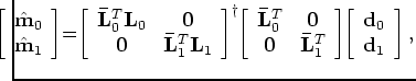$\dagger$ is the pseudo refers to the pseudo-inverse.

The RJMI method differs from separate inversion, because it enables inclusion of both spatial regularization (as in separate inversion) and temporal regularization (e.g., Tikhonov) so that the cost function becomes

$$\begin{array}{ccc} S({\bf m_{0}}, {\bf m_{1}})= \left \vert\l... ... \end{array} \right ] \right \vert \right \vert ^2, \end{array}$$ (A-15)

where ${\bf\Lambda_{i}}$ is the temporal regularization, and $\zeta_{i}$ is a relative temporal regularization parameter that determines the strength of the temporal constraint. Similar formulations have been applied to seismic tomography (Ajo-Franklin et al., 2005) and medical imaging problems (Zhang et al., 2005). However, for our problem, a direct minimization of equation 15 with an iterative solver is computationally expensive:

$$cost\propto 2 \times N_{surv} \times N_{iter} \times C_{mig},$$ (A-16)

where 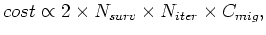$N_{surv}$ is the number of data sets, $N_{iter}$ is the number of iterations, and $C_{mig}$ is the cost of on migration. Although it is possible to reduce the computational cost by encoding the data sets (Ayeni et al., 2009), conventional single-record shot-profile implementation is too expensive for practical applications. Because several iterations are usually required to reach a useful solution, and because inversion is usually repeated several times to fine-tune parameters, the overall cost of this scheme makes it impractical. One advantage of the RJMI method is that modifications can be made to inversion parameters and the inversion repeated at several orders of magnitude more cheaply than iterative least-squares data-space migration/inversion. This cost reduction comes because the migration and modeling (demigration) operations are replaced by a single sparse-matrix convolution.

Minimizing equation 15 leads to the solutions $\hat{\bf m}_{0}$ and $\hat{\bf m}_{1}$:

$$\left [ \begin{array}{cc} \hat{\bf m}_{0} \hat{\bf m}_{1} \end... ...begin{array}{cc} \tilde {\bf m}_{0} \tilde {\bf m}_{1} \end{array} \right ],$$ (A-17)

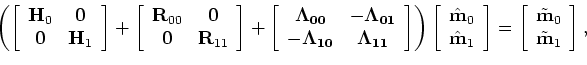
which can be obtained via iterative recursive filtering:

$$\left ( \left [ \begin{array}{ccc} {\bf H}_{0} & {\bf0} {\bf0}... ...begin{array}{cc} \tilde {\bf m}_{0} \tilde {\bf m}_{1} \end{array} \right ],$$ (A-18)

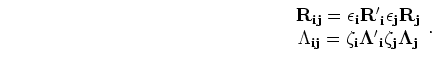
where

$$\begin{array}{ccc} {\bf R_{ij} = { {\epsilon_i R'}_i \epsilon... ...da'}_{\bf i}} \zeta_{\bf j} {\bf\Lambda_{ j}}}} \end{array} .$$ (A-19)

Following the same procedure, equation 18 can be directly extended to an arbitrary number of surveys (Ayeni and Biondi, 2008). Note that it is unnecessary to explicitly form the Hessian operators in equations 18 because they are composed of simple combinations of ${\bf H_{0}}$ to ${\bf H_{N}}$ for ${N}$ surveys. Also, ${\bf R_{ij}}$ and $\Lambda_{\bf ij}$ are not explicitly computed, but instead, the regularization operators ${\bf R_{i}}$ and ${\bf\Lambda_{\bf i}}$ (and their adjoints) are applied at each inversion step. Depending on the problem size, computational domain and available a priori information, the spatial and temporal regularization operators can be applied over several dimensions (e.g., stacked-image, subsurface offset, subsurface scattering-angles, etc.). We have implemented these operators for any arbitrary number of surveys using sparse convolution operators. Unless otherwise stated, equation 19 is solved with a conjugate gradient algorithm.

Target-oriented joint inversion of incomplete time-lapse seismic data sets