Wave-equation tomography using image-space phase-encoded data

image-space phase-encoded wavefields

The randomly encoded areal source and areal receiver wavefields can be computed as follows:

$$\left\{ \begin{array}{l} \left( \frac{\partial}{\partial z}-i \La... ... {\widetilde Q}_D(x,y,z=z_{\rm max},{\bf p}_m,\omega) = 0 \end{array} \right.,$$ (16)

and

$$\left\{ \begin{array}{l} \left( \frac{\partial}{\partial z}-i\Lam... ... {\widetilde Q}_U(x,y,z=z_{\rm max},{\bf p}_m,\omega) = 0 \end{array} \right.,$$ (17)

where $\widetilde{I}_D({\bf x},{\bf h},{\bf p}_m,\omega)$ and $\widetilde{I}_U({\bf x},{\bf h},{\bf p}_m,\omega)$ are the encoded SODCIGs. They are defined as:

$$\begin{array}{l} \widetilde{I}_D({\bf x},{\bf h},{\bf p}_m,\o... ... = \sum_{x_m,y_m}I_U({\bf x},{\bf h},x_m,y_m)\beta, \end{array}$$ (18)

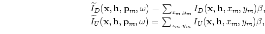where $\beta=e^{i\gamma({\bf x},x_m,y_m,{\bf p}_m,\omega)}$ is chosen to be the random phase-encoding function, with $\gamma({\bf x},x_m,y_m,{\bf p}_m,\omega)$ being a uniformly distributed random sequence in ${\bf x}$, $x_m$, $y_m$ and $\omega$; the variable ${\bf p}_m$ is the index of different realizations of the random sequence. Recursively solving Equations 16 and 17 gives us the encoded areal source data ${\widetilde Q}_D({\bf x},{\bf p}_m,\omega)$ and encoded areal receiver data ${\widetilde Q}_U({\bf x},{\bf p}_m,\omega)$, which can be collected at any depth.

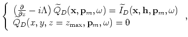
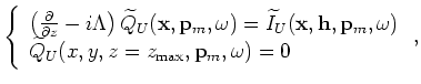
In image-space wave-equation tomography, the image-space phase-encoded areal data sets are downward continued using the one-way wave equation. The background image is produced by cross-correlating the two wavefields and summing images for all realizations ${\bf p}_m$, as follows:

$$\begin{array}{l} I_{\rm me}({\bf x},{\bf h}) = \sum_{{\bf p}_... ..._m,\omega)} \widetilde{U}({\bf x},{\bf p}_m,\omega).\end{array}$$ (19)

The initial condition for modeling simultaneous events is set by regularly selecting SODCIGs in the prestack image. The amount of crosstalk in the image $I_{\rm me}({\bf x},{\bf h})$ can be controlled by choosing a convenient sampling interval for SODCIGs used simultaneously for the modeling. For instance, if only one reflector is present and the correct velocity is used, no crosstalk is generated if the SODCIG interval is greater than twice the maximum subsurface offset of the prestack image. In the extreme case, when an incorrect velocity is used and the reflector's energy spreads through the whole range of subsurface offsets, crosstalk is not generated if the the SODCIG interval is greater than four times the maximum subsurface offset. In the presence of more than one reflector, crosstalk between reflectors occurs, regardless of the distance between SODCIGs input to modeling. By phase-encoding the reflectors, we can mitigate the crosstalk.

To phase-encode the reflectors it is necessary to pick some significant reflectors in the prestack migrated data. This implies a horizon-based approach for the prestack exploding-reflector modeling. In velocity-model updating, the idea of using some key reflectors to extract the residual-moveout information is an established strategy (Stork, 1992; Kosloff et al., 1996; Jiao et al., 2008).

The perturbed image is obtained by applying the chain rule to Equation 19. The slowness perturbation is computed by applying the adjoint of the tomographic operator, ${\bf T}^\ast$, to the image perturbation.

Wave-equation tomography using image-space phase-encoded data