|
|
|
|
Wave-equation tomography using image-space phase-encoded data |
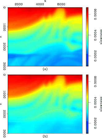
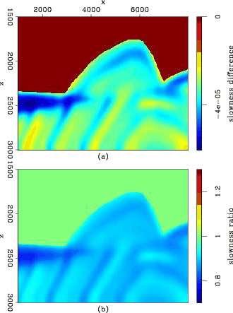
Figure 2(a) shows the true slowness model. The background velocity model is equal to the correct velocity model above 2400 m depth and above the anticline with apex at (x = 6000 m, z = 1850m). Therefore, the slowness perturbation is zero in this portion of the model. Below these horizons, the background model is characterized by a smoother version of the original Marmousi model, computed with a 400 m 2D-median filter and scaled down by a factor of ![]() . Figure 2(b) shows the background slowness. By using this background slowness model, we assume that a layer striping approach has been used and that the model is accurately defined up to a certain horizon, as usually occurs in projects of velocity model building. The slowness perturbation, computed by taking the difference between the correct and background slownesses, is shown in Figure 3(a). In the part where the slowness perturbation is different from zero, the ratio between the true and the background slowness ranges approximately from 0.8 to 0.92 (Figure 3(b)). Notice that the minimum depth is 1500 m. Henceforth, all the figures will be displayed with a minimum depth of 1500 m.
. Figure 2(b) shows the background slowness. By using this background slowness model, we assume that a layer striping approach has been used and that the model is accurately defined up to a certain horizon, as usually occurs in projects of velocity model building. The slowness perturbation, computed by taking the difference between the correct and background slownesses, is shown in Figure 3(a). In the part where the slowness perturbation is different from zero, the ratio between the true and the background slowness ranges approximately from 0.8 to 0.92 (Figure 3(b)). Notice that the minimum depth is 1500 m. Henceforth, all the figures will be displayed with a minimum depth of 1500 m.
|
|---|
|
islow
Figure 2. a) Correct slowness; b) Background slowness.[ER] |
|
|
|
|---|
|
dslow
Figure 3. a) Slowness perturbation; b) Ratio between the true and the background slownesses.[ER] |
|
|
To compute the image-space phase-encoded data, we picked ![]() reflectors in the non-zero slowness perturbation part, in the prestack image computed with the
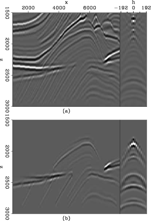
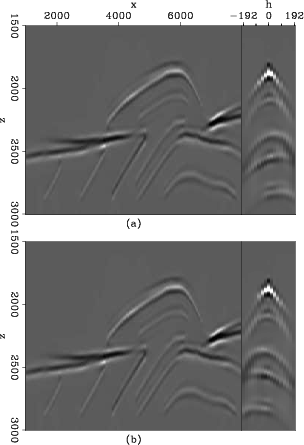
reflectors in the non-zero slowness perturbation part, in the prestack image computed with the ![]() original shots using the background slowness model. Figure 4 shows the background image (Figure 4a) computed with shot-profile migration. The panel on the left corresponds to the zero-subsurface-offset section, and the panel on the right is the SODCIG at CMP position 5500 m. Notice the effects of using an inaccurate background slowness. The reflector at (7000 m, 2500 m) is pulled up, as are the subjacent reflectors. In the SODCIG, the energy is not focused at the zero subsurface offset.
original shots using the background slowness model. Figure 4 shows the background image (Figure 4a) computed with shot-profile migration. The panel on the left corresponds to the zero-subsurface-offset section, and the panel on the right is the SODCIG at CMP position 5500 m. Notice the effects of using an inaccurate background slowness. The reflector at (7000 m, 2500 m) is pulled up, as are the subjacent reflectors. In the SODCIG, the energy is not focused at the zero subsurface offset.
Figure 4(b) shows the picked reflectors used to model the image-space phase-encoded data. This image is used as input for the rotation of the reflectors in the SODCIGs with respect to the apparent geological dip, and the results are used as the initial conditions to model the image-space phase-encoded data, as discussed by Biondi (2007,2006). Figure 5 shows the initial conditions for the prestack modeling. Figure 5(a) shows the initial condition for modeling the receiver wavefield, and Figure 5(b) shows the initial condition for modeling the source wavefield.
|
|---|
|
bimg1
Figure 4. Zero-subsurface offset section (panel on the left) and SODCIG at 5500 m (panel on the right) showing: a) background image, and b) windowed image used to compute image-space-encoded data.[CR] |
|
|
Two image-space phase-encoded data sets were synthesized using different parameters. One contains one random realization of phase-encoded areal shots initiated simultaneously with SODCIG sampling interval of 264 m and encoded according to the CMP position and reflector number, generating ![]() areal shot gathers. The other data set corresponds to two random realizations modeled with SODCIG sampling interval of 840 m, composed of
areal shot gathers. The other data set corresponds to two random realizations modeled with SODCIG sampling interval of 840 m, composed of ![]() areal shot gathers. Because in the velocity inversion we consider the maximum subsurface offset to be 192 m, this data set is expected to generate less crosstalk. In some comparisons, we use just one random realization (
areal shot gathers. Because in the velocity inversion we consider the maximum subsurface offset to be 192 m, this data set is expected to generate less crosstalk. In some comparisons, we use just one random realization (![]() areal shots) of the second data set. We use the two random realizations when comparing the results of the non-linear optimization of the slowness model. Henceforth, the image-space phase-encoded data sets are called areal shots.
areal shots) of the second data set. We use the two random realizations when comparing the results of the non-linear optimization of the slowness model. Henceforth, the image-space phase-encoded data sets are called areal shots.
|
|---|
|
rimg1
Figure 5. Zero-subsurface offset section (panel on the left) and SODCIG at 5500 m (panel on the right) showing: a) initial condition for modeling the receiver wavefield, and b) initial condition for modeling the source wavefield.[CR] |
|
|
| (20) |
 with respect to the slowness
To guarantee smoothness of the wave-equation tomography gradient, we use a B-spline representation with nodes located every 960 m in the  -direction and 16 m in the
 ![]() -direction.
-direction.
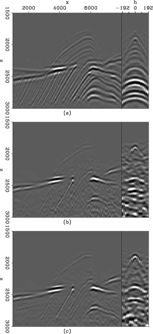
Figure 6 shows the image perturbation computed by applying the forward tomographic operator, ![]() , and using the background slowness of Figure 2(b) and the known slowness perturbation of Figure 3. Figure 6a shows the image perturbation computed in the shot-profile domain for the
, and using the background slowness of Figure 2(b) and the known slowness perturbation of Figure 3. Figure 6a shows the image perturbation computed in the shot-profile domain for the ![]() shots; Figure 6b shows the image perturbation computed in the image-space phase-encoded domain using 11 areal shots; and Figure 6c shows the image perturbation computed in the image-space phase-encoded domain using 35 areal shots. Notice that the dispersed crosstalk is stronger in Figure 6b than in Figure 6c.
shots; Figure 6b shows the image perturbation computed in the image-space phase-encoded domain using 11 areal shots; and Figure 6c shows the image perturbation computed in the image-space phase-encoded domain using 35 areal shots. Notice that the dispersed crosstalk is stronger in Figure 6b than in Figure 6c.
|
|---|
|
dimg1
Figure 6. Zero-subsurface offset section (panel on the left) and SODCIG at 5500 m (panel on the right) showing: a) image perturbation in the shot-profile domain; b) image perturbation computed with |
|
|
Figure 7 illustrates the normalized slowness perturbations obtained by applying the adjoint tomographic operator
![]() to the image perturbations of Figure 6. Compare with the correct slowness perturbation of Figure 3. Figure 7a is the predicted slowness perturbation found by back-projecting Figure 6a using all
to the image perturbations of Figure 6. Compare with the correct slowness perturbation of Figure 3. Figure 7a is the predicted slowness perturbation found by back-projecting Figure 6a using all ![]() shot gathers; Figure 7b shows the back-projection of Figure 6b using
shot gathers; Figure 7b shows the back-projection of Figure 6b using ![]() areal shots; and Figure 7c shows the back-projection of Figure 6c using
areal shots; and Figure 7c shows the back-projection of Figure 6c using ![]() areal shots. Notice that we do not use a B-spline representation for the slowness perturbations. In general, the predicted slowness perturbation with image-space phase-encoded gathers shows a structure similar to that obtained with the original shot gathers. The differences can be credited, at first order, to the occurrence of residual crosstalk in the image-space phase-encoded perturbed image and to a sub-optimal number of selected reflectors for the prestack exploding-reflector modeling.
areal shots. Notice that we do not use a B-spline representation for the slowness perturbations. In general, the predicted slowness perturbation with image-space phase-encoded gathers shows a structure similar to that obtained with the original shot gathers. The differences can be credited, at first order, to the occurrence of residual crosstalk in the image-space phase-encoded perturbed image and to a sub-optimal number of selected reflectors for the prestack exploding-reflector modeling.
|
|---|
|
dsadj
Figure 7. Normalized slowness perturbation obtained by applying the adjoint tomographic operator |
|
|
Finally, we compare the optimized slowness models with the correct slowness model of Figure 2(a). After 5 non-linear iterations for both the ![]() areal shots and
areal shots and ![]() areal shots (one random realization) of the
areal shots (one random realization) of the ![]() -gather image-space phase-encoded data set the optimization stopped because the difference between the objective functional of successive iterations was smaller than the machine precision. The number of function evaluations was 28 for the
-gather image-space phase-encoded data set the optimization stopped because the difference between the objective functional of successive iterations was smaller than the machine precision. The number of function evaluations was 28 for the ![]() areal shots, and 27 for the
areal shots, and 27 for the ![]() areal shots. We also computed 2 non-linear iterations with a total of 6 function evaluations using the two random realizations of the
areal shots. We also computed 2 non-linear iterations with a total of 6 function evaluations using the two random realizations of the ![]() areal shots. To verify the accuracy of the resulting optimized slowness models, we also migrated the original shot gathers with the three optimized slownesses and also with the correct slowness.
areal shots. To verify the accuracy of the resulting optimized slowness models, we also migrated the original shot gathers with the three optimized slownesses and also with the correct slowness.
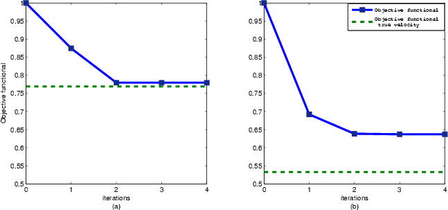
Figure 8 displays the evolution of the objective functional with the non-linear iterations for the ![]() areal shots (Figure 8(a)) and
areal shots (Figure 8(a)) and ![]() areal shots (Figure 8(b)). For comparison, the value of the objective functional for the true velocity is also shown as dashed lines. The values are normalized according to the value of the objective functional of the first iteration for each case. The objective functional was reduced in 22
areal shots (Figure 8(b)). For comparison, the value of the objective functional for the true velocity is also shown as dashed lines. The values are normalized according to the value of the objective functional of the first iteration for each case. The objective functional was reduced in 22![]() and 36
and 36![]() for the
for the ![]() areal shots and for the
areal shots and for the ![]() areal shots, respectively. Notice that those values are 23
areal shots, respectively. Notice that those values are 23![]() and 47
and 47![]() , respectively, when using the true slowness model. The smaller difference between the final optimized value of the objective functional and the objective functional computed with the true slowness model for the optimization with the
, respectively, when using the true slowness model. The smaller difference between the final optimized value of the objective functional and the objective functional computed with the true slowness model for the optimization with the ![]() areal shots, can be partially credited to the more severe crosstalk generated by this data set than the
areal shots, can be partially credited to the more severe crosstalk generated by this data set than the ![]() areal shots. Even if the correct slowness model is used, residual crosstalk is amplified when applying the DSO operator.
areal shots. Even if the correct slowness model is used, residual crosstalk is amplified when applying the DSO operator.
|
|---|
|
plot
Figure 8. Evolution of the objective functional with the non-linear iterations. The dashed lines represent the value of the objective functional for the true slowness model. a) Normalized objective functional for the |
|
|
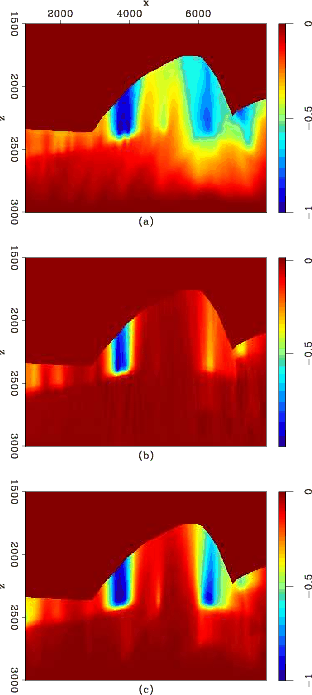
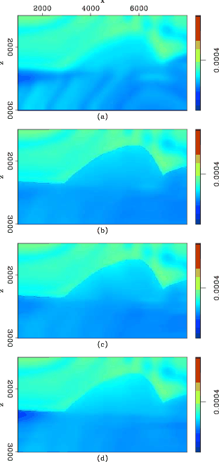
Figure 9 shows the optimized slownesses and, for comparison purposes, the true slowness. Figure 9(a) displays the slowness model; Figure 9(b) is the slowness model obtained with the ![]() -gather image-space phase encoded data; Figure 9(c) is the slowness model obtained with the
-gather image-space phase encoded data; Figure 9(c) is the slowness model obtained with the ![]() -gather image-space phase encoded data; and Figure 9(d) is the slowness model obtained with the
-gather image-space phase encoded data; and Figure 9(d) is the slowness model obtained with the ![]() -gather image-space phase encoded data. In general, the predicted slownesses are reasonable. The predicted slowness using the
-gather image-space phase encoded data. In general, the predicted slownesses are reasonable. The predicted slowness using the ![]() areal shots shows slightly lower values than the other two predicted slownesses. Notice that the detailed slowness variation present in the true slowness is not recovered in the optimized slownesses, due to the B-spline representation of the gradient of the wave-equation tomography objective functional. In addition, as we are solving for the deeper portion of the model with dipping reflectors, it is likely that deficient illumination prevents us to obtain a more accurate slowness model. However, the slowness model obtained with the
areal shots shows slightly lower values than the other two predicted slownesses. Notice that the detailed slowness variation present in the true slowness is not recovered in the optimized slownesses, due to the B-spline representation of the gradient of the wave-equation tomography objective functional. In addition, as we are solving for the deeper portion of the model with dipping reflectors, it is likely that deficient illumination prevents us to obtain a more accurate slowness model. However, the slowness model obtained with the ![]() areal shots recovers the low slowness values on the left of model better than the other two predicted slownesses.
areal shots recovers the low slowness values on the left of model better than the other two predicted slownesses.
|
|---|
|
sfperm
Figure 9. True and optimized slownesses. a) True slowness model; b) Slowness model obtained with the |
|
|
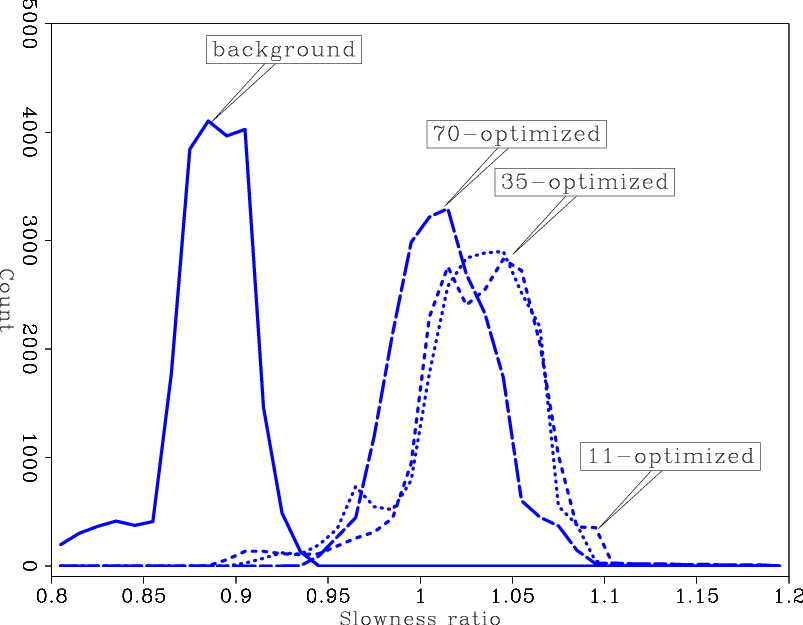
Figure 10 shows the histograms of the ratio between the true and background interval slowness (continuous line) and between the true and predicted interval slownesses obtained with the ![]() (fine dash),
(fine dash), ![]() (fine dot), and
(fine dot), and ![]() areal shots (large dash) below the depth of 2400 m.
areal shots (large dash) below the depth of 2400 m.
|
|---|
|
hsfperm
Figure 10. Histograms of the slowness ratios between the true and background interval slowness (continuous line) and between the true and predicted interval slownesses obtained with the |
|
|
The mean and standard deviation of the corresponding distributions are summarized in Table 1. In general, the predicted slownesses vary between ![]() to
to ![]() of the true slowness. The background slowness varies between
of the true slowness. The background slowness varies between ![]() to
to ![]() of the true slowness.
of the true slowness.
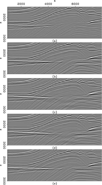
Figure 11 displays the zero-subsurface-offset section after migration of the ![]() original shot gathers using the true slowness model (Figure 11(b)), the predicted slowness using
original shot gathers using the true slowness model (Figure 11(b)), the predicted slowness using ![]() areal shots (Figure 11(c)), the predicted slowness using
areal shots (Figure 11(c)), the predicted slowness using ![]() areal shots (Figure 11(d)), and the predicted slowness using
areal shots (Figure 11(d)), and the predicted slowness using ![]() areal shots (Figure 11(e)). For comparison, we also display in Figure 11(a) the zero-subsurface-offset section after migration with the background slowness of Figure 2(b). Notice that reflectors in the central portion of Figure 11(a) are pulled up when comparing to Figure 11(b). The image obtained with the optimized slowness model computed with the
areal shots (Figure 11(e)). For comparison, we also display in Figure 11(a) the zero-subsurface-offset section after migration with the background slowness of Figure 2(b). Notice that reflectors in the central portion of Figure 11(a) are pulled up when comparing to Figure 11(b). The image obtained with the optimized slowness model computed with the ![]() areal shots (Figure 11(c))presents pushed down reflectors around (4000 m, 2500 m) as a consequence of the lower values of the optimized slowness. In addition, in this image the undulating character of the reflector at (7000 m, 2600 m) reflects some velocity inaccuracy, when compared to Figures 11(b) and (e).
areal shots (Figure 11(c))presents pushed down reflectors around (4000 m, 2500 m) as a consequence of the lower values of the optimized slowness. In addition, in this image the undulating character of the reflector at (7000 m, 2600 m) reflects some velocity inaccuracy, when compared to Figures 11(b) and (e).
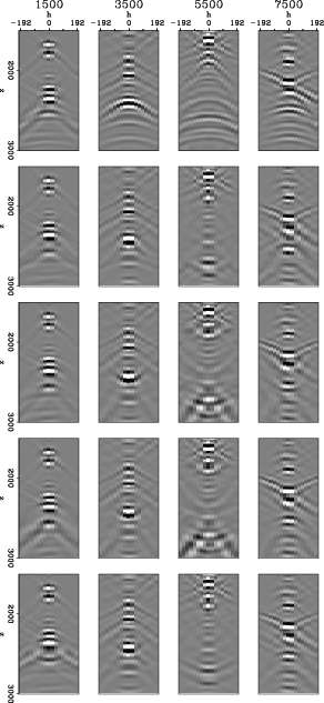
From top to bottom, Figure 12 displays SODCIGs at 1500 m, 3500 m, 5500 m and 7500 m after migration of the ![]() original shot gathers, using the background slowness of Figure 2(b) in the first row, using the true slowness model in the second row, using the predicted slowness with
original shot gathers, using the background slowness of Figure 2(b) in the first row, using the true slowness model in the second row, using the predicted slowness with ![]() areal shots in the third row, using the predicted slowness with
areal shots in the third row, using the predicted slowness with ![]() areal shots in the fourth row, and using the predicted slowness with
areal shots in the fourth row, and using the predicted slowness with ![]() areal shots in the fifth row. The subsurface-offset ranges from -192 m to 192 m. The analysis of the SODCIGs in Figures 12(c) to (e) shows that better focusing is achieved when more image-space phase-encoded gathers are used in the wave-equation tomography.
areal shots in the fifth row. The subsurface-offset ranges from -192 m to 192 m. The analysis of the SODCIGs in Figures 12(c) to (e) shows that better focusing is achieved when more image-space phase-encoded gathers are used in the wave-equation tomography.
|
|---|
|
fimg1
Figure 11. Zero-subsurface-offset section after migration of the |
|
|
|
|---|
|
fimg11
Figure 12. Subsurface-offset gathers after migration of the |
|
|
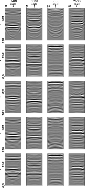
Figure 13 displays the angle-domain common-image gathers (ADCIGs) taken at the same CMP position as SODCIGs of Figure 12. From top to bottom, Figure 13 displays ADCIGs after migration using the background slowness in the first row, using the true slowness model in the second row, using the predicted slowness with ![]() areal shots in the third row, using the predicted slowness with
areal shots in the third row, using the predicted slowness with ![]() areal shots in the fourth row, and using the predicted slowness with
areal shots in the fourth row, and using the predicted slowness with ![]() areal shots in the fifth row. Notice that migration with the predicted slowness using
areal shots in the fifth row. Notice that migration with the predicted slowness using ![]() areal shots shows virtually no residual moveout. For the case of predicted slowness using
areal shots shows virtually no residual moveout. For the case of predicted slowness using ![]() and
and ![]() areal shots some residual moveout occurs for CMP position 5500 m. As can be seen if Figure 13, the angular coverage for the dipping deep reflectors we consider in the slowness inversion ranges from
areal shots some residual moveout occurs for CMP position 5500 m. As can be seen if Figure 13, the angular coverage for the dipping deep reflectors we consider in the slowness inversion ranges from
![]() to
to
![]() . For the reflectors at the central portion of the model it varies between
. For the reflectors at the central portion of the model it varies between
![]() to
to
![]() . This limited angular coverage decreases the resolution of the slowness estimate.
. This limited angular coverage decreases the resolution of the slowness estimate.
|
|---|
|
fang1
Figure 13. ADCIGs after angle transformation of the SODCIGs of Figure 12. From top to bottom: in the first row, using the background slowness model; the second row, using the true slowness model; in the third row, using the predicted slowness model of Figure 9(b); in the fourth row, using the predicted slowness model of Figure 9(c); and in the fifth row, using the predicted slowness model of Figure 9(d).[CR] |
|
|
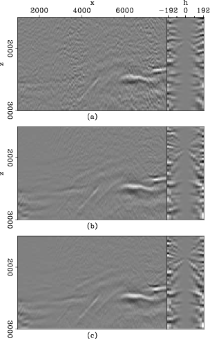
The accuracy of the optimized slowness improves when using more phase-encoded gathers in the wave-equation tomography, or, in other words, when the crosstalk in the perturbed image is less severe, as Figures 6 and 7 suggest. Figure 14 shows the perturbed image computed by applying the DSO operator on the image migrated with the background slowness of Figure 2(b). The panel on the left corresponds to the subsurface-offset -144 m and the panel on the right is the SODCIG taken at 5500 m. Figure 14(a) shows the perturbed image using ![]() areal shots; Figure 14(b) shows the perturbed image using
areal shots; Figure 14(b) shows the perturbed image using ![]() areal shots; and Figure 14(c) shows the perturbed image using
areal shots; and Figure 14(c) shows the perturbed image using ![]() areal shots. Notice how the signal-to-noise ratio improves as more phase-encoded gathers are used. The SODCIG of the perturbed image of Figure 14(a) presents coherent events, related to unattenuated crosstalk, curving upward at z = 2700 m; these events are not present in Figures 14(b) and (c). If these events are sufficiently incoherent along the subsurface-offset sections, a two-dimensional filter could be applied to attenuate them. In that case, a new objective function should be defined. This deserves future investigation.
areal shots. Notice how the signal-to-noise ratio improves as more phase-encoded gathers are used. The SODCIG of the perturbed image of Figure 14(a) presents coherent events, related to unattenuated crosstalk, curving upward at z = 2700 m; these events are not present in Figures 14(b) and (c). If these events are sufficiently incoherent along the subsurface-offset sections, a two-dimensional filter could be applied to attenuate them. In that case, a new objective function should be defined. This deserves future investigation.
|
|---|
|
dso
Figure 14. Perturbed images computed with the DSO operator. a) Perturbed image using |
|
|
|
|
|
|
Wave-equation tomography using image-space phase-encoded data |