|
|
|
|
Measuring image focusing for velocity analysis |
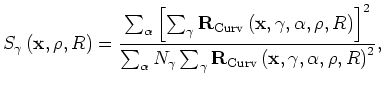
Figure 14 shows the reflectors' geometry assumed to model the two synthetic data sets. I modeled the first data set assuming a "cloud" of point diffractors (panel a), whereas I modeled the second data set assuming a "cloud" of convex reflectors (panel b). In both cases the velocity was assumed to be constant and equal to 2 km/s and the data were migrated assuming a high slowness of .5125 s/km; that is, 102.5% of the correct slowness.
Figure 15 summarizes
the main result of this section.
All three panels show the image-focusing
semblance spatially averaged in an inner rectangle of the image space
defined by the following inequalities along the depth axis:
 ,
and
by the following inequalities along the midpoint axis:
,
and
by the following inequalities along the midpoint axis:
![]() x
x
![]() .
The panel shows the average semblance as a function of the
velocity parameter
.
The panel shows the average semblance as a function of the
velocity parameter ![]() and the radius of curvature
and the radius of curvature ![]() .
Figure 15a shows the result corresponding to
the point diffractors and
Figure 15b shows the result corresponding to
the convex reflectors.
In both cases,
I applied the curvature correction defined in 5
by using a field of local dips (
.
Figure 15a shows the result corresponding to
the point diffractors and
Figure 15b shows the result corresponding to
the convex reflectors.
In both cases,
I applied the curvature correction defined in 5
by using a field of local dips (
 ) estimated numerically
by applying the Seplib program Sdip to the ensemble
of residual migrated images for each value of
) estimated numerically
by applying the Seplib program Sdip to the ensemble
of residual migrated images for each value of ![]() .
.
The important observation supported by this figure
is that,
in both Figure 15a
and Figure 15b,
the semblance energy is concentrated
in a relatively narrow interval that includes
the correct value of ![]() ;
that is
;
that is
![]() .
This result indicates that we can extract useful velocity information
from zero-offset data by using the image-focusing semblance.
.
This result indicates that we can extract useful velocity information
from zero-offset data by using the image-focusing semblance.
The third panel in Figure 15,
shows the semblance average computed from the images
of the convex reflectors when I applied the
curvature correction defined in 5
by using a constant local dip equal to zero; that is,
when I uniformly set
![]() .
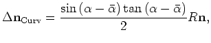
As predicted by expression 9,
there is strong ambiguity between the reflector
curvature and the velocity parameter and the semblance
is high also for values of
.
As predicted by expression 9,
there is strong ambiguity between the reflector
curvature and the velocity parameter and the semblance
is high also for values of ![]() that are far away from the correct one.
We can consequently conclude
that the velocity information contained in panel a) and b)
derives from the inconsistency between
the focusing information extracted using the image-focusing semblance
and the local dip estimation.
This inconsistency occurs
when the image is sufficiently unfocused that the local dip
estimation becomes unreliable.
The following figures illustrate this concept.
that are far away from the correct one.
We can consequently conclude
that the velocity information contained in panel a) and b)
derives from the inconsistency between
the focusing information extracted using the image-focusing semblance
and the local dip estimation.
This inconsistency occurs
when the image is sufficiently unfocused that the local dip
estimation becomes unreliable.
The following figures illustrate this concept.
Figures 16-20
provide a graphical explanation of the results shown in
Figure 15.
Figure 16 shows the migrated
images of the point-diffractors data corresponding to the
values of ![]() at the edges of the semblance peak in
Figure 15a.
The inner rectangle delimited by the grid superimposed
to the images shows where the semblance is spatially averaged
to produce the results shown in
Figure 15.
The image in Figure 16a is undermigrated
and corresponds to
at the edges of the semblance peak in
Figure 15a.
The inner rectangle delimited by the grid superimposed
to the images shows where the semblance is spatially averaged
to produce the results shown in
Figure 15.
The image in Figure 16a is undermigrated
and corresponds to
![]() ,
whereas the image in Figure 16b
is overmigrated and corresponds to
,
whereas the image in Figure 16b
is overmigrated and corresponds to
![]() .
In both of these images the unfocusing starts to cause crossing
of events in the inner rectangle delimited by the grid superimposed
to the images.
The local dips are then multivalued and the automatic
estimation of the local dips becomes unreliable and inconsistent with the
more global behavior of the dips.
Therefore, outside the interval
.
In both of these images the unfocusing starts to cause crossing
of events in the inner rectangle delimited by the grid superimposed
to the images.
The local dips are then multivalued and the automatic
estimation of the local dips becomes unreliable and inconsistent with the
more global behavior of the dips.
Therefore, outside the interval
![]() the semblance average drops substantially in value.
the semblance average drops substantially in value.
Similar behavior is displayed by
the migrated
images of the convex-reflectors data corresponding to the
values of ![]() at the edges of the semblance peak in
Figure 15a.
These images are shown in Figure 17,
and correspond to
at the edges of the semblance peak in
Figure 15a.
These images are shown in Figure 17,
and correspond to ![]() (Figure 17a),
and to
(Figure 17a),
and to ![]() (Figure 17b).
In this case,
the
(Figure 17b).
In this case,
the ![]() range is wider than in the previous case
because the convex-reflectors' density is lower than
the point-diffractors' density,
and thus a larger velocity error is needed before
poorly focused events start crossing.
range is wider than in the previous case
because the convex-reflectors' density is lower than
the point-diffractors' density,
and thus a larger velocity error is needed before
poorly focused events start crossing.
Figures 18-20
show sections cut through
the image-focusing semblance cubes at constant value
of ![]() and
and ![]() before spatial averaging.
Figure 18a shows semblance
for the point-diffractors data for
before spatial averaging.
Figure 18a shows semblance
for the point-diffractors data for
![]() and
and ![]() meters;
that is, the values of
meters;
that is, the values of ![]() and
and ![]() for which the data are best focused.
Figure 18a shows semblance
for
for which the data are best focused.
Figure 18a shows semblance
for
![]() and
and ![]() meters.
This value of
meters.
This value of ![]() is the one corresponding to the undermigrated image in
Figure 16a.
Because of undermigration,
the image from the point diffractors appears to have a positive
radius of curvature approximately equal to 40 m.
However, because of inconsistency between the focusing
information and the local dip estimation,
semblance is in average lower in the panel on the right
than in the panel on the left.
is the one corresponding to the undermigrated image in
Figure 16a.
Because of undermigration,
the image from the point diffractors appears to have a positive
radius of curvature approximately equal to 40 m.
However, because of inconsistency between the focusing
information and the local dip estimation,
semblance is in average lower in the panel on the right
than in the panel on the left.
Similar behavior is displayed by
the image-focusing semblance cubes computed from
the images of the convex-reflectors data.
We find the ``best focused'' semblance panel
(Figure 19a)
still at infinite curvature (![]() meters),
but at a wrong value of
meters),
but at a wrong value of ![]() ; that is, at
; that is, at ![]() .
However, the important result is that the interval
with relative high semblance still includes the correct
value of
.
However, the important result is that the interval
with relative high semblance still includes the correct
value of ![]() .
The section shown in
Figure 19b corresponds
to undermigrated image
shown in Figure 19b,
and it is taken for
.
The section shown in
Figure 19b corresponds
to undermigrated image
shown in Figure 19b,
and it is taken for ![]() and
and ![]() meters.
The apparent curvature is lower than
for the point diffractors because the actual curvature
of the reflector is lower.
meters.
The apparent curvature is lower than
for the point diffractors because the actual curvature
of the reflector is lower.
Finally, Figure 20
shows sections through the image-focusing semblance cubes for
the convex-reflectors data when the local dip is uniformly set equal to zero.
These panels correspond to the average semblance shown in
Figure 15c,
and are sections taken for the same values of ![]() and
and ![]() as the sections shown in Figure 17.
Because of the ambiguity between velocity and curvature,
both panels show well-focused and high
value semblance peaks.
as the sections shown in Figure 17.
Because of the ambiguity between velocity and curvature,
both panels show well-focused and high
value semblance peaks.
|
Refl-all-overn
Figure 14. Reflectors' geometry assumed to model the two zero-offset synthetic data sets I used to test the proposed image-focusing velocity-estimation method: a) a "cloud" of point diffractors, and b) a "cloud" of convex reflectors. [ER] |

|
|---|---|
|
|

|
|---|
|
Wind-Stack-all-overn
Figure 15. The image-focusing semblance spatially averaged in an inner rectangle of the image space as a function of velocity parameter |
|
|
|
ResMig-all-scatter-overn
Figure 16. Migrated images of the point-diffractors data corresponding to the values of |

|
|---|---|
|
|
|
ResMig-all-repl-bump-overn
Figure 17. Migrated images of the convex-reflectors data corresponding to the values of |

|
|---|---|
|
|
|
Wind-Sembl-scatter-all-overn
Figure 18. Sections cut through the image-focusing semblance cubes at constant value of |

|
|---|---|
|
|
|
Wind-Sembl-repl-bump-all-overn
Figure 19. Sections cut through the image-focusing semblance cubes at constant value of |

|
|---|---|
|
|
|
Wind-Sembl-repl-bump-dip-0-all-overn
Figure 20. Sections cut through the image-focusing semblance cubes at constant value of |

|
|---|---|
|
|
|
|
|
|
Measuring image focusing for velocity analysis |