|
|
|
|
Measuring image focusing for velocity analysis |
 is the local dip and .
To estimate the local dips,
I used the Seplib program Sdip that implements
a variant of the algorithms described by Fomel (2002).
is the local dip and .
To estimate the local dips,
I used the Seplib program Sdip that implements
a variant of the algorithms described by Fomel (2002).
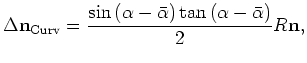
Expression 2 can be used directly to create an
ensemble to dip-decomposed images that are corrected for the local
curvature
![]() .
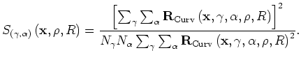
The image-focusing semblance can be computed
on these images as:
.
The image-focusing semblance can be computed
on these images as:
However, the application of correction 2
can be quite expensive unless it is performed together with residual migration.
Furthermore, precomputing the curvature-corrected images
would further increase
the dimensionality of the image space, creating obvious problems
for handling the resulting bulky data sets.
Fortunately, when the ensemble of
the dip-decomposed images
![]() are the result of residual prestack migration,
the curvature correction can be efficiently
computed during the evaluation of the semblance
functional 3.
Correction 2 becomes a simple interpolation
along the residual velocity parameter
are the result of residual prestack migration,
the curvature correction can be efficiently
computed during the evaluation of the semblance
functional 3.
Correction 2 becomes a simple interpolation
along the residual velocity parameter ![]() , as a function
of the aperture angles and dips.
, as a function
of the aperture angles and dips.
To derive the interpolating function, I first recall the expression of residual migration in Biondi (2008a):
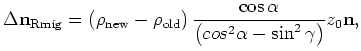 is the normal shift applied by residual migration,
Equating the normal shift in 4 with the normal shift
in 2 and solving for
![]() we obtain
we obtain
![$\displaystyle {\bf R}_{{\rm Curv}}\left({\bf x},\gamma ,\alpha ,\rho_{\rm old},...
...o_{\rm new}\left(\rho_{\rm old},\gamma ,\alpha ,\bar{\alpha},{R}\right)\right].$](img38.png) |
(A-6) |
|
|
|
|
Measuring image focusing for velocity analysis |