Attribute combinations for image segmentation

Eigenvector combinations

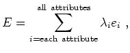
Finally, a third approach is to use the individual attribute volumes to calculate multiple eigenvectors, and then combine the eigenvectors before determining a boundary. Following the recommendation of Shi and Malik (2000), a simple way to combine the eigenvectors is via linear combination:

$$E = \sum_{i=\mathrm{each \ attribute}}^{\mathrm{all \ attributes}} \lambda_i e_i \ ,$$ (3)

where $e_i$ is an individual eigenvector and $\lambda_i$ is a specific weight value assigned to the attribute in question. Of course, taking this approach introduces the problem of determining weight values for each attribute. Panel (c) in Figure 4 shows the result of this approach if equal weights are given to the amplitude and dip attributes. While the boundary is satisfactory in many locations, the dip attribute clearly has too much influence in some areas where the amplitude attribute provides much better information. This method shows promise, but a mechanism for assigning better weights is necessary. One such mechanism has already been discussed; we can use the eigenvector uncertainty measurement, utilized previously for the boundary combination approach, to assign attribute weight values for a linear combination of eigenvectors. In this way, we are able to follow the recommendation of Shi and Malik for combining information from different sources, while at the same time taking advantage of a ``built-in'' method for estimating uncertainties.

Since the eigenvectors range in value from -1 to +1, the eigenvector difference across one of the boundaries can never be greater than two. Thus, the value

$$\omega = \frac{1}{2} (1+d_{amp} - d_{dip}) \ ,$$ (4)

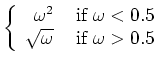
where $d$ is the difference across a calculated boundary at a particular 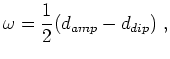$x$ location, will range from 0 to 1. If we want to heavily penalize uncertainty in one of the eigenvectors, we set the weight values as follows:

$$W_{amp} = \left\{ \begin{array}{rl} \omega^2 &\mbox{ if $\omega < 0.5$} \\ \sqrt{\omega} &\mbox{ if $\omega > 0.5$} \end{array} \right.$$ (5)

$$W_{dip} = 1 - w_{amp} .$$ (6)

The results of assigning weight values in this manner to create an eigenvector are shown in panel (d) of Figure 4. The boundary successfully follows the salt interface everywhere the amplitude-only boundary does, and incorporates the dip information only where the amplitude boundary fails. Furthermore, we do not see the erratic behavior in areas where the dip information is most significant, as we did for the boundary combination method.

Attribute combinations for image segmentation