Attribute combinations for image segmentation

Attribute combinations

In the segmentation algorithm, the determination of a salt interface takes place in three distinct stages. The first stage is the calculation of attributes that may be useful in indicating a boundary between sediments and a salt body. The second stage involves transforming the attribute volumes into eigenvectors of the image via the construction of a weight matrix based on the attribute values. Finally, the third stage ``draws" the salt boundary using the eigenvector values. Each of these three stages represents an opportunity for combining information from different attributes. The following sections will explore these three options, and illustrate their advantages and disadvantages with example calculations on a 2D seismic section taken from a 3D Gulf of Mexico field dataset, seen in Figure 1.

dat
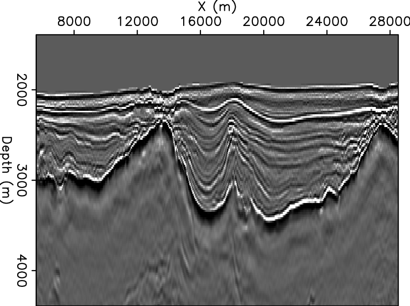
Figure 1. A migrated seismic section used for 2D segmentation examples. Note the discontinous nature of the strong reflector (salt boundary), which will present challenges for the segmentation algorithm. [ER]

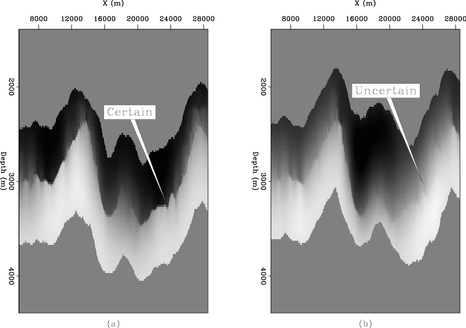
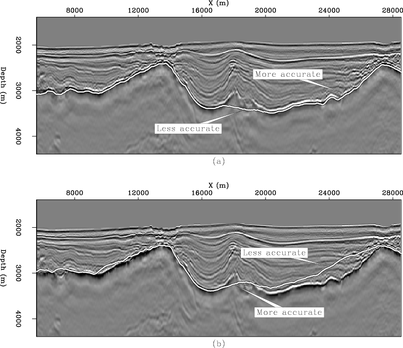
The following examples will seek to combine useful information from two attributes - amplitude and dip variability. Figure 2 shows eigenvectors derived from these two individual attributes. The eigenvector values range from -1 to +1; in the figures here, negative values are dark and positive values are light. The salt boundary is typically drawn along the zero-contour of the eigenvector, where values pass from negative to positive. Thus, a sharp transition from dark to light colors in the eigenvector indicates a boundary location with relative certainty, while a grey area indicates a slower transition from negative to positive values, and relative uncertainty of the boundary location. Clearly, the amplitude eigenvector provides better information throughout most of the image, although the transition near $x=18000$ suggests significant uncertainty. This is logical, as the original section (Figure 1) shows a great deal on discontinuity at this location. Overall, the dip eigenvector shows much less certainty than the one derived from the amplitude attribute; however, the previously mentioned location appears more certain on the dip eigenvector. The boundary calculations corresponding to these two eigenvectors (Figure 3) confirm these observations. Therefore, an obvious goal for combining information from these two attributes is to produce a boundary that uses information from the amplitude attribute in most locations, but incorporates the dip information at this location.

eigs-ann
Figure 2. Eigenvectors derived from amplitude of the envelope (a) and dip variability (b) attributes. Areas of relative boundary certainty and uncertainty are indicated. [CR]

ampdipbnd
Figure 3. Zero-contour boundaries corresponding to the amplitude (a) and dip variability (b) eigenvectors seen in Figure 2. [CR]

Attribute combinations for image segmentation