Attribute combinations for image segmentation

Boundary combinations

A second ``domain'' in which information from different attributes may be combined is after individual boundary calculations have already taken place. This method requires a measure of uncertainty along each individual boundary, so that a new boundary can be created by incorporating the ``most certain'' boundary at each location in the image. As discussed previously, such an uncertainty measure may be gleaned from the zero-crossing of the eigenvector:

$$d = \vert p_1 - n_1\vert ,$$ (2)

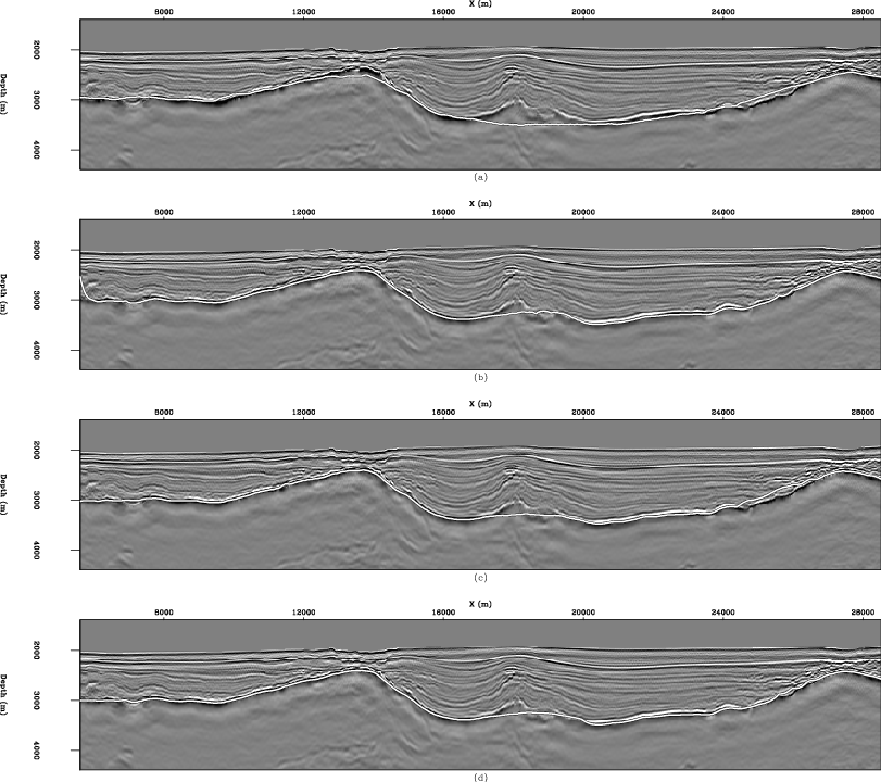
where $p_1$ and $n_1$ are the two values on either side of the boundary (one will be positive, one negative). A sharp transition from positive to negative values - quantitatively, a large value of $d$ at that location - signifies relative certainty, while a slow transition or small difference signals uncertainty. In this case, the measurement is taken perpendicular to the calculated boundary, so as to avoid the assumption that the boundary is in all locations locally horizontal. After such calculations are made at all locations for each boundary, a combined boundary is formed by taking the most certain boundary location (depth value) at each horizontal location. Panel (b) in Figure 4 shows the result of this process.

This approach performs very well in this example. Information from the amplitude attribute is honored nearly everywhere, and the dip information is incorporated only where it is superior to the amplitude information. However, the manner in which this approach is implemented could lead to problems in some circumstances. Taking the best elements of different boundaries could easily lead to erratic, ``either/or'' behavior in the combined boundary; indeed, some indications of this behavior may be seen in the jaggedness of the boundary where the dip information plays a significant role. It is likely that this behavior would be even more troublesome in three dimensions.

uno-bnds
Figure 4. Calculated boundaries corresponding to: (a) Attribute multiplication segmentation; (b) Combination of individual boundaries; (c) Equally-weighted eigenvector combination; and (d) Uncertainty-weighted eigenvector combination. [CR]

Attribute combinations for image segmentation