|
 |
 |
 | Image-space wave-equation tomography in the generalized source domain |  |
![[pdf]](icons/pdf.png) |
Next: Numerical examples
Up: tomography with the encoded
Previous: Data-space encoded wavefields
The image-space encoded gathers are obtained using
the prestack exploding-reflector modeling method introduced by Biondi (2006) and Biondi (2007).
The general idea of this method is to model the data and the corresponding source function that are related to only one event in
the subsurface, where a single unfocused SODCIG (obtained with an inaccurate velocity model)
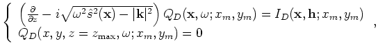
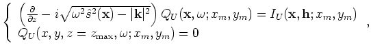
is used as the initial condition for the recursive upward
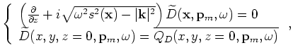
continuation with the following one-way wave equations:
 |
|
|
(A-28) |
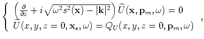
and
 |
|
|
(A-29) |
where
 and
and
 are the isolated SODCIGs at the horizontal location
  for a single reflector, and are suitable for the initial conditions
for the source and receiver wavefields, respectively.
They are obtained by rotating the original unfocused SODCIGs
according to the apparent geological dip of the reflector.
This rotation maintains the velocity information
needed for migration velocity analysis, especially for dipping reflectors (Biondi, 2007).
By collecting the wavefields at the surface, we obtain the areal source data
for a single reflector, and are suitable for the initial conditions
for the source and receiver wavefields, respectively.
They are obtained by rotating the original unfocused SODCIGs
according to the apparent geological dip of the reflector.
This rotation maintains the velocity information
needed for migration velocity analysis, especially for dipping reflectors (Biondi, 2007).
By collecting the wavefields at the surface, we obtain the areal source data
 and the areal receiver data
 for a single reflector and a single SODCIG located at .
Since the size of the migrated image volume can be very big in practice and there are usually many reflectors in the
subsurface, modeling each reflector and each SODCIG one by one may generate a data set even bigger
than the original data set. One strategy to reduce the cost is to model several reflectors and several SODCIGs
simultaneously (Biondi, 2006); however, this process generates unwanted crosstalk.
As discussed by Guerra and Biondi (2008a,b), random phase encoding
could be used to attenuate the crosstalk.
The randomly encoded areal source and areal receiver wavefields can be computed as follows:
 |
|
|
(A-30) |
and
 |
|
|
(A-31) |
where
 and
and
 are the encoded SODCIGs after rotations. They are defined as follows:
where
 is chosen to be the random phase-encoding function,
with
is chosen to be the random phase-encoding function,
with
 being a uniformly distributed random sequence in
  ,
,  ,
,  and
and  ;
the variable
;
the variable  is the index of different realizations of the random sequence.
Recursively solving Equations 30 and 31 gives us the encoded
areal source data
is the index of different realizations of the random sequence.
Recursively solving Equations 30 and 31 gives us the encoded
areal source data
 and areal receiver data
 , which can be collected on the surface.
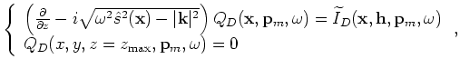
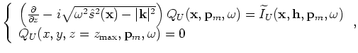
The synthesized new data sets are downward continued using the same one-way wave equation defined
by Equations 13 and 14 (with different boundary conditions) as follows:
 |
|
|
(A-34) |
and
 |
|
|
(A-35) |
where
 and
and
 are the downward continued areal source
and areal receiver wavefields for realization .
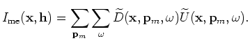
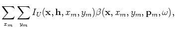
The image is produced by cross-correlating the two wavefields and summing images for all realization as follows:
are the downward continued areal source
and areal receiver wavefields for realization .
The image is produced by cross-correlating the two wavefields and summing images for all realization as follows:
 |
|
|
(A-36) |
The crosstalk artifacts can be further attenuated if the number of is large; therefore, approximately,
the image obtained by migrating the image-space encoded gathers is kinematically equivalent to the image obtained in the shot-profile domain.
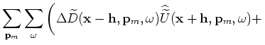
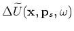
From Equation 36, the perturbed image is easily obtained as follows:
where
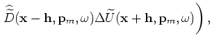 and
and
 are the image-space encoded background source and receiver wavefields;
 and
and
 are the perturbed source and receiver wavefields
in the image-space phase-encoding domain, which satisfy the perturbed one-way wave equations defined by Equations 17 and 18.
The tomographic operator
are the perturbed source and receiver wavefields
in the image-space phase-encoding domain, which satisfy the perturbed one-way wave equations defined by Equations 17 and 18.
The tomographic operator  and its adjoint
 can be implemented in a manner similar to that discussed in Appendices B and C, by
replacing the original wavefields with the image-space phase-encoded wavefields.
can be implemented in a manner similar to that discussed in Appendices B and C, by
replacing the original wavefields with the image-space phase-encoded wavefields.
|
|
|
|
| Image-space wave-equation tomography in the generalized source domain | |
|
Next: Numerical examples
Up: tomography with the encoded
Previous: Data-space encoded wavefields
2009-04-13