|
 |
 |
 | Image-space wave-equation tomography in the generalized source domain |  |
![[pdf]](icons/pdf.png) |
Next: tomography with the encoded
Up: Image-space wave-equation tomography in
Previous: image-space wave-equation tomography
For the conventional shot-profile migration, both source and receiver wavefields are downward continued with the
following one-way wave equations (Claerbout, 1971):
 |
|
|
(A-13) |
and
 |
|
|
(A-14) |
where the overline stands for complex conjugate;
 is the source wavefield for a single frequency
  at image point
 with the source located at
 ;
;
 is the
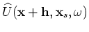
receiver wavefield for a single frequency at image point
is the
receiver wavefield for a single frequency at image point  for the source located at
  ;
;
 is the slowness at ;
 is the spatial wavenumber vector;
 is the frequency dependent source signature, and
 defines the point source function at ,
which serves as the boundary condition of Equation 13.
defines the point source function at ,
which serves as the boundary condition of Equation 13.
 is the recorded shot gather for the shot located at ,
which serves as the boundary condition of Equation 14.
To produce the image, the following cross-correlation imaging condition is used:
is the recorded shot gather for the shot located at ,
which serves as the boundary condition of Equation 14.
To produce the image, the following cross-correlation imaging condition is used:
 |
|
|
(A-15) |
where
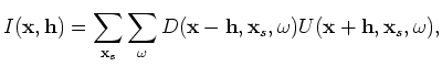 is the subsurface half offset.
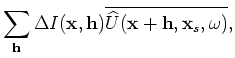
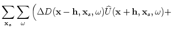
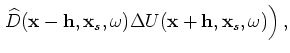
The perturbed image can be derived by a simple application of the chain rule
to Equation 15:
where
 and
and
 are the background source and
receiver wavefields computed with the background slowness
are the background source and
receiver wavefields computed with the background slowness
 ;
;
 and
and
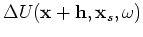
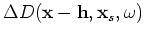 are the perturbed source wavefield and perturbed receiver wavefield, which are the results of the slowness perturbation
 .
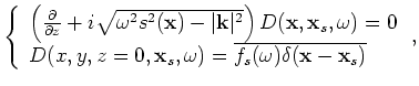
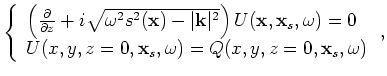
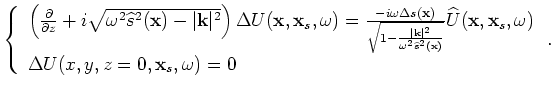
The perturbed source and receiver wavefields satisfy the following
one-way wave equations, which are linearized with respect to slowness (see Appendix A for derivations):
.
The perturbed source and receiver wavefields satisfy the following
one-way wave equations, which are linearized with respect to slowness (see Appendix A for derivations):
 |
|
|
(A-17) |
and
 |
|
|
(A-18) |
Recursively solving Equations 17 and 18 gives us the perturbed source and receiver wavefields.
The perturbed source and receiver wavefields are then used in Equation 16 to generate the perturbed image
 , where
the background source and receiver wavefields are precomputed by recursively solving Equations 13 and 14 with a
background slowness
, where
the background source and receiver wavefields are precomputed by recursively solving Equations 13 and 14 with a
background slowness
 .
Appendix B gives a more detailed matrix representation of how to evaluate the forward tomographic operator
.
Appendix B gives a more detailed matrix representation of how to evaluate the forward tomographic operator  .
.
To evaluate the adjoint tomographic operator  , we first apply the adjoint of the imaging condition in Equation 16
to get the perturbed source and receiver wavefields
, we first apply the adjoint of the imaging condition in Equation 16
to get the perturbed source and receiver wavefields
 and
and
 as follows:
Then we solve the adjoint equations of Equations 17 and 18 to get the slowness perturbation
.
Again, in order to solve the adjoint equations of Equations 17 and 18,
the background source wavefield
 and
the background receiver wavefield
and
the background receiver wavefield
 have to be computed in advance.
Appendix C gives a more detailed matrix representation of how to evaluate the adjoint tomographic operator
have to be computed in advance.
Appendix C gives a more detailed matrix representation of how to evaluate the adjoint tomographic operator
 .
.
|
|
|
|
| Image-space wave-equation tomography in the generalized source domain | |
|
Next: tomography with the encoded
Up: Image-space wave-equation tomography in
Previous: image-space wave-equation tomography
2009-04-13