 |
 |
 |
 | Image-space wave-equation tomography in the generalized source domain |  |
![[pdf]](icons/pdf.png) |
Next: the tomographic operator in
Up: Image-space wave-equation tomography in
Previous: introduction
Image-space wave-equation tomography is a non-linear inverse problem
that tries to find an optimal background slowness that minimizes the residual field,
 , defined in the image space.
The residual field is derived from the background image,
, defined in the image space.
The residual field is derived from the background image,  , which is computed with a background slowness (or the current estimate of the slowness).
The residual field measures the correctness of the background slowness;
its minimum (under some norm, e.g.
, which is computed with a background slowness (or the current estimate of the slowness).
The residual field measures the correctness of the background slowness;
its minimum (under some norm, e.g.  ) is achieved when a correct background slowness has been used for migration.
There are many choices of the residual field, such as residual moveout in the Angle-Domain Common-Image Gathers (ADCIGs),
differential semblance in the ADCIGs,
reflection-angle stacking power (in which case we have to maximize the residual field, or minimize the negative stacking power), etc..
Here we follow a definition similar to that in Biondi (2008), and define a general form of the residual field as follows:
) is achieved when a correct background slowness has been used for migration.
There are many choices of the residual field, such as residual moveout in the Angle-Domain Common-Image Gathers (ADCIGs),
differential semblance in the ADCIGs,
reflection-angle stacking power (in which case we have to maximize the residual field, or minimize the negative stacking power), etc..
Here we follow a definition similar to that in Biondi (2008), and define a general form of the residual field as follows:
 |
|
|
(A-1) |
where  is a focusing operator, which measures the focusing of the migrated image. For example,
in the Differential Semblance Optimization (DSO) method (Shen, 2004), the focusing operator takes the following form:
is a focusing operator, which measures the focusing of the migrated image. For example,
in the Differential Semblance Optimization (DSO) method (Shen, 2004), the focusing operator takes the following form:
 |
|
|
(A-2) |
where  is the identity operator and
  is the DSO operator either in the subsurface offset domain or in the angle domain (Shen, 2004).
The subsurface-offset-domain DSO focuses the energy at zero offset, whereas the angle-domain DSO flattens the ADCIGs.
is the DSO operator either in the subsurface offset domain or in the angle domain (Shen, 2004).
The subsurface-offset-domain DSO focuses the energy at zero offset, whereas the angle-domain DSO flattens the ADCIGs.
In the wave-equation migration velocity analysis (WEMVA) method (Sava, 2004), the focusing operator is the linearized residual migration operator defined as follows:
![$\displaystyle {\bf F}({\bf I}) = {\bf R}[\rho]{\bf I} \approx {\bf I} + {\bf K}[\Delta \rho]{\bf I},$](img16.png) |
|
|
(A-3) |
where  is the ratio between the background slowness
 and the true slowness
  ,
and
,
and
 ;
;
![$ {\bf R}[\rho]$](img21.png) is the residual migration operator (Sava, 2003), and
is the residual migration operator (Sava, 2003), and
![$ {\bf K}[\Delta \rho]$](img22.png) is the differential residual migration operator defined as follows (Sava and Biondi, 2004a,b):
is the differential residual migration operator defined as follows (Sava and Biondi, 2004a,b):
![$\displaystyle {\bf K}[\Delta \rho] = \Delta \rho \left. \frac{\partial {\bf R}[\rho]}{\partial \rho} \right\vert _{\rho=1}.$](img23.png) |
|
|
(A-4) |
The linear operator
applies different phase rotations to the image for different reflection angles and geological dips (Biondi, 2008).
In general, if we choose norm, the tomography objective function to minimize can be written as follows:
 |
|
|
(A-5) |
where
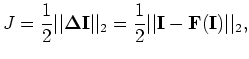 stands for the norm.
Gradient-based optimization techniques such as the quasi-Newton method and the conjugate gradient method can be used to minimize the objective function
stands for the norm.
Gradient-based optimization techniques such as the quasi-Newton method and the conjugate gradient method can be used to minimize the objective function  .
The gradient of with respect to the slowness reads as follows:
.
The gradient of with respect to the slowness reads as follows:
 |
|
|
(A-6) |
where 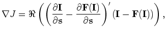 denotes taking the real part of a complex value and
  denotes the adjoint.
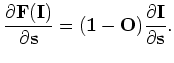
For the DSO method, the linear operator is independent of the slowness,
so we have
denotes the adjoint.
For the DSO method, the linear operator is independent of the slowness,
so we have
 |
|
|
(A-7) |
Substituting Equations 2 and 7 into Equation 6 and evaluating the gradient at a background slowness yields
 |
|
|
(A-8) |
where
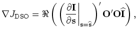 is the background image computed using the background slowness
.
is the background image computed using the background slowness
.
For the WEMVA method, the gradient is slightly more complicated, because in this case, the focusing operator is also dependent
on the slowness . However, one can simplify it by assuming that the focusing operator is applied on the background
image
instead of , and
 is also picked from the background image
, that is
is also picked from the background image
, that is
![$\displaystyle {\bf F}(\widehat{\bf I})=\widehat{\bf I}+{\bf K}[\widehat{\Delta \rho}]\widehat{\bf I}.$](img34.png) |
|
|
(A-9) |
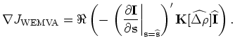
With these assumptions, we get the "classic" WEMVA gradient as follows:
![$\displaystyle \nabla J_{\rm WEMVA} = \Re \left( - \left.\left(\frac{\partial {\...
...t{\bf s}}\right)^{\prime}{\bf K}[\widehat{\Delta \rho}]\widehat{\bf I} \right).$](img35.png) |
|
|
(A-10) |
The complete WEMVA gradient without the above assumptions can also be derived following the method described by Biondi (2008).
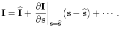
No matter which gradient we choose to back-project the slowness perturbation, we have to evaluate the adjoint of the linear operator
 , which defines a linear mapping from
the slowness perturbation
, which defines a linear mapping from
the slowness perturbation
 to the image perturbation
. This is easy to see by
expanding the image around the background slowness
to the image perturbation
. This is easy to see by
expanding the image around the background slowness
 as follows:
 |
|
|
(A-11) |
Keeping only the zero and first order terms, we get the linear operator
as follows:
 |
|
|
(A-12) |
where
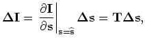 and
and
 .
.
 is the wave-equation tomographic operator.
The tomographic operator can be evaluated either in the source and receiver domain (Sava, 2004) or in the shot-profile domain (Shen, 2004).
In next section we follow an approach similar to that discussed by Shen (2004) and review the forward and adjoint tomographic operator
in the shot-profile domain. In the subsequent sections, we generalize the expression of the tomographic operator to
the generalized source domain.
is the wave-equation tomographic operator.
The tomographic operator can be evaluated either in the source and receiver domain (Sava, 2004) or in the shot-profile domain (Shen, 2004).
In next section we follow an approach similar to that discussed by Shen (2004) and review the forward and adjoint tomographic operator
in the shot-profile domain. In the subsequent sections, we generalize the expression of the tomographic operator to
the generalized source domain.
|
|
|
|
| Image-space wave-equation tomography in the generalized source domain | |
|
Next: the tomographic operator in
Up: Image-space wave-equation tomography in
Previous: introduction
2009-04-13