Examples with synthetic data

As a first example, I will consider the synthetic dataset shown in panel (a) of Figure 1. There are two primaries (black) and four multiples (white). The traveltimes of both primaries and multiples were computed analytically from a three flat-layer model: water layer, a sedimentary layer and a half space. The estimates of the multiples (b) and primaries (c) were computed by adding 40% of the primaries to the multiples and 40% of the multiples to the primaries, respectively. The goal is to simulate a situation in which the kinematics of the estimates of primaries and multiples are both correct but there is strong cross-talk (leakage) between them.

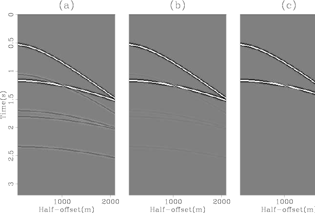
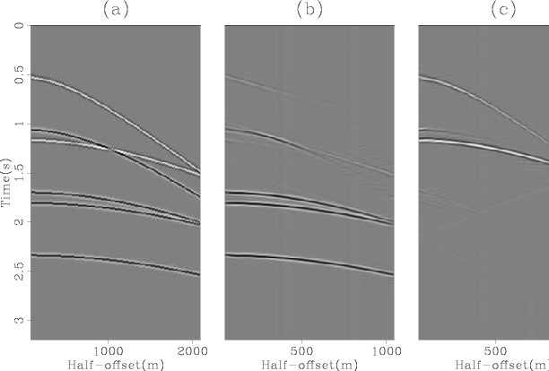
Figure 2 shows the estimated multiples after one, two and three outer iterations of the algorithm. The corresponding results for the estimated primaries are shown in Figure 3. In both figures we see that the cross-talk is substantially reduced after the first outer iteration and is completely eliminated after the third. Notice the hole in the top multiple and the bottom primary in the final estimates. This is actually present in the data (panel (a) in Figure 1) and is an artifact because both primaries and multiples were modeled with the same amplitude and opposite polarity.

syn1-estimates1
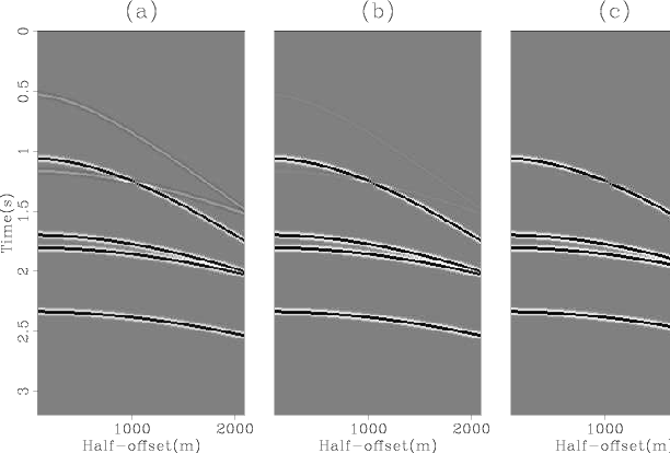
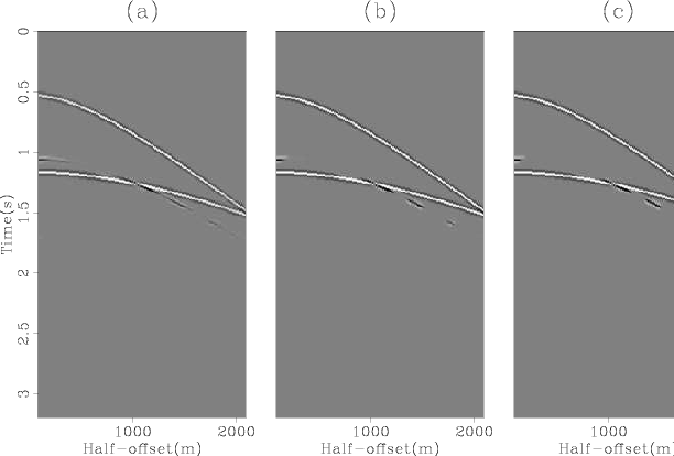
Figure 1. Synthetic CMP gather (a) showing two primaries (black) and four multiples (white) from a three flat-layer model. The initial estimates of multiples (b) and primaries (c) are contaminated with 40% cross-talk.

syn1-matched-muls
Figure 2. Matched estimates of multiples after one (a), two (b) and three (c) outer iterations of the algorithm.

syn1-matched-prims
Figure 3. Matched estimates of primaries after one (a), two (b) and three (c) outer iterations of the algorithm.

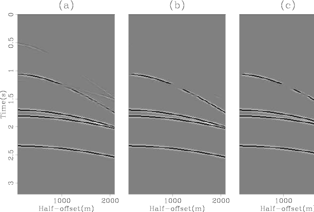
Consider now the more realistic situation of kinematic and offset-dependent amplitude errors in the original estimates of both primaries and multiples, as well as noise as shown in Figure 4. The multiple and primary estimates were obtained via migration-demigration as described in (). These are imperfect estimates with cross-talk on primaries and multiples and other noises.

syn2-estimates1
Figure 4. Original CMP gather (a), initial estimate of the multiples (b) and initial estimate of the primaries (c).

Panel (a) of Figures 5 and 6 show the results after one outer iteration, whereas panels (b) and (c) of the same figures show the results after three and five outer iterations respectively. There is still some localized cross-talk from the multiples into the primaries.

syn2-matched-muls
Figure 5. Matched estimates of multiples after one (a), three (b) and five (c) outer iterations of the algorithm.

syn2-matched-prims
Figure 6. Matched estimates of primaries after one (a), three (b) and five (c) outer iterations of the algorithm.

The next example uses the well-known Sigsbee model (, ) to illustrate the method in the image space. For this example, therefore, ``data'' means the migrated image with primaries and multiples. This dataset has the advantage that, along with the modeled data (primaries and multiples), there exists a related dataset without the free surface multiples (http://www.delphi.tudelft.nl/SMAART/S2Breadme.htm). Panel (a) of Figure 7 shows the modeled data, panel (b) the data without free surface multiples (b), and panel (c) the estimated free surface multiples in the image space computed with an image space version of SRME (, ). All panels are plotted at the exact same clip value. Notice that the estimate of the multiples is accurate only in kinematics, not in amplitudes or frequency content. The estimate of the multiples was computed with an image space version of SRME (, ).

sgsb-estimates1
Figure 7. Sigsbee migrated dataset. Data (a), migrated model without surface multiples (b) and initial estimates of multiples (c).

In contrast with the previous examples, in this case I do not have an independent initial estimate of the primaries. I could subtract the estimate of the multiples from the data, but the corresponding estimate of the primaries is too distorted. Using such a poor primary estimate actually hurts the chances of matching the multiples to the data. Another option is to use the data itself as the initial estimate of the primaries. I found, however, that a better alternative is to do a first iteration setting $\mu=0$, meaning only the multiples need to be matched. Once matched, the multiples are subtracted from the data to get the estimate of the primaries for the next iteration.

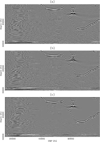
Figures 8 and 9 show a close-up view of the matched primaries and multiples, respectively, after one, two and three outer iterations. After the first iteration, the most obvious multiples contaminating the estimate of the primaries have been attenuated (compare panels (a) of Figures 7 and 8) but strong residual multiple energy remains. The second iteration helps attenuate the multiples further, although it is hard to appreciate in these small figures. See, for example the multiple inside the salt and in the bottom right corner of panel (b). The third iteration cleans up most of the noise, although it also weakens the subsalt primaries.

sgsb-matched-prims
Figure 8. Estimated primaries after one (a), two (b) and three (c) outer iterations of the algorithm.

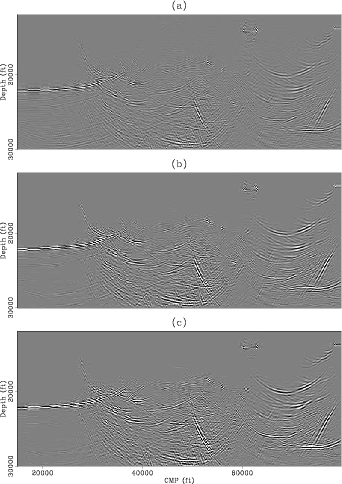
sgsb-matched-muls
Figure 9. Estimated multiples after one (a), two (b) and three (c) outer iterations of the algorithm.

On the estimate of the multiples, again the first iteration extracts the most significant multiples and the second iteration locally corrects the amplitudes. The third iteration actually hurts the estimate of the multiples because the effect of the regularization term becomes significant as the match of both the primaries and the multiples to the data improves. The net result is an estimate of the primaries that is close to the primaries in the original image. Because of the need for regularization, the estimate of the multiples, however, is weaker than it should.