Next: Examples with synthetic data
Up: Adaptive matching
Previous: Introduction
Conceptually, the first step of the new method is to form the convolutional
matrices of both the estimated multiples  and the estimated primaries
 . In practice, these are huge matrices that are not explicitly formed
but are replaced by equivalent linear operators (, ). Next, I compute
non-stationary filters in
micro-patches (that is, filters that act locally on overlapping two-dimensional
partitions of the data) to match the estimated multiples and the estimated
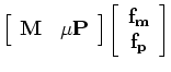
primaries, to the data containing both. I compute the filters by solving the
following linear least-squares inverse problem:
. In practice, these are huge matrices that are not explicitly formed
but are replaced by equivalent linear operators (, ). Next, I compute
non-stationary filters in
micro-patches (that is, filters that act locally on overlapping two-dimensional
partitions of the data) to match the estimated multiples and the estimated
primaries, to the data containing both. I compute the filters by solving the
following linear least-squares inverse problem:
where  and
and  are the matching filters for the
multiples and
primaries respectively,
are the matching filters for the
multiples and
primaries respectively,  is a parameter to balance the relative
importance of the two components of the fitting goal (, ),
is a parameter to balance the relative
importance of the two components of the fitting goal (, ),
 is
the data (primaries and multiples),
is
the data (primaries and multiples),  is a regularization
operator, (in my implementation a Laplacian operator), and
is a regularization
operator, (in my implementation a Laplacian operator), and  is the
usual parameter to control the level of regularization.
is the
usual parameter to control the level of regularization.
Once convergence is achieved, each filter is applied to its corresponding
convolutional matrix, and new estimates for and are computed:
Here  represents the index of the outer iteration of the linear problem
described by Equations 1 and 2. Notice that I hold constant
although it could be changed from iteration to iteration
represents the index of the outer iteration of the linear problem
described by Equations 1 and 2. Notice that I hold constant
although it could be changed from iteration to iteration  . Also notice
that the regularization operator
. Also notice
that the regularization operator  and the regularization parameter
in Equation 2 could be different for and .
I have chosen to keep them the same to limit the number of adjustable parameters.
This choice worked very well in all my tests.
The updated versions of the convolutional matrices
and the regularization parameter
in Equation 2 could be different for and .
I have chosen to keep them the same to limit the number of adjustable parameters.
This choice worked very well in all my tests.
The updated versions of the convolutional matrices
 and
and
 are plugged into equations 1 and 2 and the
process repeated until the cross-talk has been eliminated or significantly attenuated.
are plugged into equations 1 and 2 and the
process repeated until the cross-talk has been eliminated or significantly attenuated.
Next: Examples with synthetic data
Up: Adaptive matching
Previous: Introduction
2007-10-24